Spatial and Temporal Patterns of Groundwater Levels: A Case Study of Alluvial Aquifers in the Murray–Darling Basin, Australia

Abstract

Understanding the temporal patterns in groundwater levels and their spatial distributions is essential for quantifying the natural and anthropogenic impacts on groundwater resources for better management and planning decisions. The two most popular clustering analysis methods in the literature, hierarchical clustering analysis and self-organizing maps, were used in this study to investigate the temporal patterns of groundwater levels from a dataset with 910 observation bores in the largest river system in Australia. Results showed the following: (1) Six dominant cluster patterns were found that could explain the temporal groundwater trends in the Murray–Darling Basin. Interpretation of each of these patterns indicated how groundwater in each cluster behaved before, during, and after the Millennium Drought. (2) The two methods produced similar results, indicating the robustness of the six dominant patterns that were identified. (3) The Millennium Drought, from 1997 to 2009, had a clear impact on groundwater level temporal variability and trends. An example causal attribution analysis based on the clustering results (using a neural network model to represent groundwater level dynamics) is introduced and will be expanded in future work to identify drivers of temporal and spatial changes in groundwater level for each of the dominant patterns, leading to possibilities for better water resource understanding and management.

1. Introduction

Groundwater is an essential freshwater resource, with half of all drinking water worldwide and 43% of irrigation water at a global scale being sourced from aquifers [1,2]. Many aquifers in the world have been overused in the last several decades due to regional development and population growth. This has resulted in a series of problems, such as declining groundwater levels, land subsidence, deterioration of groundwater quality, decrease or loss of streamflow/springs, and threats to groundwater-dependent ecosystems and some endangered species which rely on groundwater for survival at different temporal and spatial scales [2,3,4,5,6,7].

Assessment of groundwater resources over time is critical for understanding natural and anthropogenic impacts on groundwater resources as well as developing appropriate management policies [8,9,10]. Given the complexity of groundwater systems (i.e., not easily accessible, hidden underground, high residence times [10,11,12,13]), the most popular metric employed to assess these resources is groundwater level, which is measured using dedicated monitoring networks [10]. Trends and variabilities observed in groundwater levels over time reflect the aggregation of the effect of multiple hydrological processes (e.g., groundwater recharge, evapotranspiration, extraction, surface water–groundwater interactions, among others) acting at different spatial and temporal scales and driven by human activities and/or climate variability [8,10]. Trend analyses are therefore useful in evaluating where groundwater levels are stable, increasing or decreasing, which indicates the status of the resource and provides an evidence base for management decisions [9,10].

There are many studies that have investigated the temporal patterns of groundwater levels. For example, Bennett et al. [14] assessed the spatial and temporal variability of groundwater levels in the shallow aquifer system on the flanks of Mount Meru, Northern Tanzania, and found that there is a rise of about 1.80 m between the static water levels in April 2018 and December 2020 on the north-eastern flank of the mountain, but a decrease of about 0.50 m between the static water levels in May 2018 and December 2020 on the western flank due to low and reduced recharge. Yin et al. [15] undertook hierarchical clustering of groundwater levels for regional groundwater drought assessment in the San Joaquin River Basin, California, and concluded that long-term (40-year) temporal patterns in groundwater levels varied significantly. They found statistically significant decreasing trends for more than 35% of wells with an average decline of 0.69 m/year mainly driven by heavy groundwater exploitation. Marchant et al. [16] developed a modeling framework for regional groundwater drought analysis based on temporal interpolation of groundwater level hydrographs. They used linear mixed models to account for seasonal variation, long-term trends, and responses to precipitation and temperature over different temporal scales. Naranjo-Fernández [17] used k-means (static) and time series (dynamic) clustering techniques to obtain different clusters of groundwater levels in the Almonte-Marismas aquifer of southwest Spain, which were associated with diverse levels of water exploitation depending on soil and hydrogeological settings.

However, different temporal patterns in groundwater level within a time window may result in similar magnitudes of overall trends due to varied groundwater processes and mechanisms affecting groundwater levels in distinct parts of the time window. This results from the complex behavior of aquifers that is influenced by a variety of factors such as rainfall, evaporation, hydrology, geology, atmospheric pressure fluctuations, tides, earthquakes, and human activities including, but not limited to, direct groundwater extraction, land use and land cover change, managed aquifer recharge and drainage [14,18]. Hence, it is required to investigate and unpack the trends in space and time to gain more insights.

Clustering analyses are often used to identify and classify patterns in trends. Clark [19] performed a self-organizing map clustering analysis of historical temporal groundwater patterns in the Namoi Basin of Australia to identify common pattern information that is shared across time series that was then used as input for groundwater level prediction models. Wu et al. [18] have investigated the spatial and temporal patterns of groundwater in Kaohsiung City using hierarchical clustering analysis and found that the clustering results are not only consistent with lithology distributions and the age of sedimentary layer but also provide newer insights on aquifer response to recharge–discharge phenomena.

A previous study [10] investigated groundwater level trends in the alluvial aquifers of the Murray–Darling Basin (MDB), Australia’s largest river basin covering an area of more than 1 million km² [10]. Long–term trends of groundwater level declines were observed for 90–95% of groundwater bores, of which 84–87% are statistically significant at α = 0.05. In contrast, 7–9% of groundwater bores showed an increasing trend of groundwater level, possibly reflecting local conditions associated with localized recharge due to surface water interactions or irrigation. It was noted that these dominant trends are more pronounced in specific resource units than in others. The sustainable diversion limit (SDL) resource unit is the name used in Australia to define a surface water or groundwater management area within the MDB with a long-term annual average limit on how much water can be used for consumptive purposes.

In this study, two cluster analysis techniques, classical hierarchical clustering and unsupervised self-organizing map (SOM) clustering, are performed to investigate the spatial and temporal patterns of groundwater levels in the MDB. The study helps to improve the understanding of groundwater level trends by addressing the following questions: What are the dominant temporal patterns in groundwater level trends in the MDB? Is there a spatial configuration for these patterns? What was the impact of the Millennium Drought (a severe and prolonged dry period from 1997 to 2009 [20]) on groundwater level patterns? How robust are these patterns to different clustering techniques? Would it be possible to identify drivers of groundwater level change for the different patterns?

Answers to these questions are critical not only for understanding natural and anthropogenic impacts on groundwater resources, but also for groundwater management and planning purposes.

2. Materials and Methods

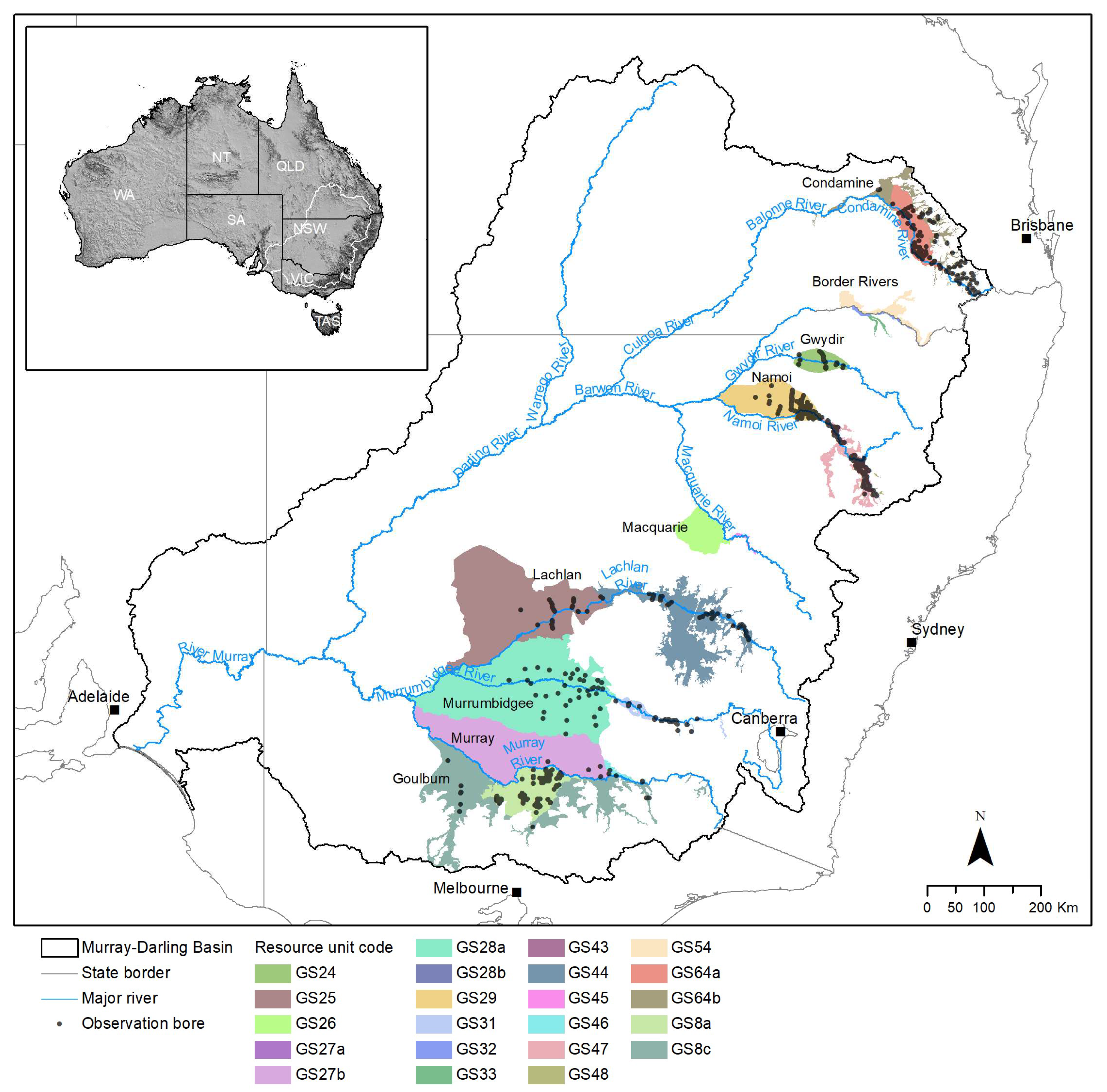
2.1. Study Region

The Murray–Darling Basin (MDB) (Figure 1) is the largest and most important river system in Australia [10]. It covers 1,060,000 km² or roughly one seventh of the Australian continent, spanning five federated states, and is home to about 2 million people in addition to providing the potable water supply to another 1 million outside the basin [10]. The MDB is considered the “food bowl” of Australia [21], with almost all of Australia’s rice and close to 90% of its cotton being produced in the basin [21], as well as other major crops, such as cereals, grapes, and horticulture [22]. The climate in the MDB varies from sub-tropical in the north to Mediterranean in the south, alpine in the south-east, and semi-arid in the west. The mean annual rainfall, areal potential evapotranspiration, and runoff averaged over the entire MDB are 457, 1443, and 27 mm, respectively [10]. There is a clear east–west rainfall gradient, where rainfall is highest in the south-east (mean annual rainfall of more than 1500 mm) and along the eastern perimeter and lowest in the west (less than 300 mm) [23,24].

The focus region of this study is limited to the eight large alluvial aquifer systems (Figure 1) within the MDB for two reasons: almost all long-term groundwater level observation bores are located in these aquifers and about 75% of total metered groundwater use is from these alluvial systems [10]. A location map is provided in Figure 1, showing the MDB basin boundary, the resource units, and the locations of the groundwater measurement bores.

2.2. Datasets

2.2.1. Groundwater Level Data

Annual time series of groundwater levels (the depth to standing water level, or DTW) at 910 bores located in the eight large alluvial systems within the MDB are used in this study (Figure 1). The raw data is downloaded from the National Groundwater Information System (NGIS) [25] but processed after following a critical data quality control procedure [10]. The dataset includes bores with a minimum of two observations per year for at least 40 years out of the 51-year (1971–2021) study period [10].

The groundwater levels were scaled into the range [0,1] by bore to enable reasonable comparison between groundwater bores with different geographic locations, elevations, depths, and horizontal aquifer extents, with the below equation:

$$x_{sc}=\frac{x-x_{min}}{x_{max}-x_{min}}$$

(1)

where x_sc is the scaled groundwater level, x is the raw groundwater level, and x_min and x_max are the maximum and minimum values of groundwater levels at that bore.

2.2.2. Rainfall and Potential Evapotranspiration (PET)

The SILO (Scientific Information for Land Owners) data [26] that provide daily climate variables across Australia are used in this study to explore the temporal relationships between groundwater levels and climate variables, i.e., rainfall and potential evapotranspiration (PET). This dataset was interpolated from station measurements made by the Australian Bureau of Meteorology (BoM) with the smoothing, splining, and kriging techniques described in [26]. It has two versions, i.e., SILO Patched Point (a time series of data at a station location) and Data Drill (a time series of data at a 0.05 °C grid point location consisting entirely of interpolated estimates) datasets. One advantage of the SILO Data Drill is that it provides a consistent climate data set across the entire study region at every 0.05° grid (approximately 5 km × 5 km) in space without any gaps (refilling the missing data) and with a standardized data quality [27]. The data are publicly available at https://www.longpaddock.qld.gov.au/silo/ (accessed on 1 June 2022).

2.2.3. Groundwater Extraction Data

Groundwater systems across the MDB can be subdivided into four major aquifer types comprising fractured rock outcropping mainly along the eastern boundary of the basin, alluvial aquifers associated with major rivers, tertiary limestone aquifers in the western Murray Basin [10,28,29], and sediments associated with the Great Artesian Basin in the northern sub-basin [29]. This study is limited to the eight large alluvial aquifer systems (Figure 1) within the MDB for reasons discussed in Section 2.1.

The Murray–Darling Basin Authority [30] highlights that 92% of total annual actual groundwater use was metered for the year 2018–2019. Average groundwater use in the MDB for the period 2012–2013 to 2018–2019 was 1.482 × 10⁹ m³/y [10] and about 75% of total metered groundwater use is from the eight alluvial systems of this study region [10].

The metered groundwater extraction information was obtained from state government water agencies. However, data were only available from 2006 and were provided aggregated at resource unit level due to data licensing restrictions.

2.3. Cluster Analysis

2.3.1. Hierarchical Clustering

Hierarchical clustering, also called hierarchical cluster analysis (HCA), is an algorithm that seeks to build a hierarchy of groups or clusters so that each cluster is distinctive from other clusters but the elements within the same cluster are broadly similar. In this study, hierarchical clustering was used to classify groundwater monitoring bores into different groups based on similarity and differences in the water level time series data obtained for these bores. The results of hierarchical clustering can be presented as a dendrogram, which is a diagram with a tree structure representing the hierarchical relationship between elements [31]. To determine which cluster the individual element (groundwater bore in this study) belongs to, a metric is needed to measure the distance between every element and others [31]. The Euclidean Distance is the most popular choice and is used in this study. The number of groups/cluster is determined by using a threshold Euclidean Distance to produce distinct clusters. Six clusters/groups were chosen for this study based on the distances among them and their temporal patterns.

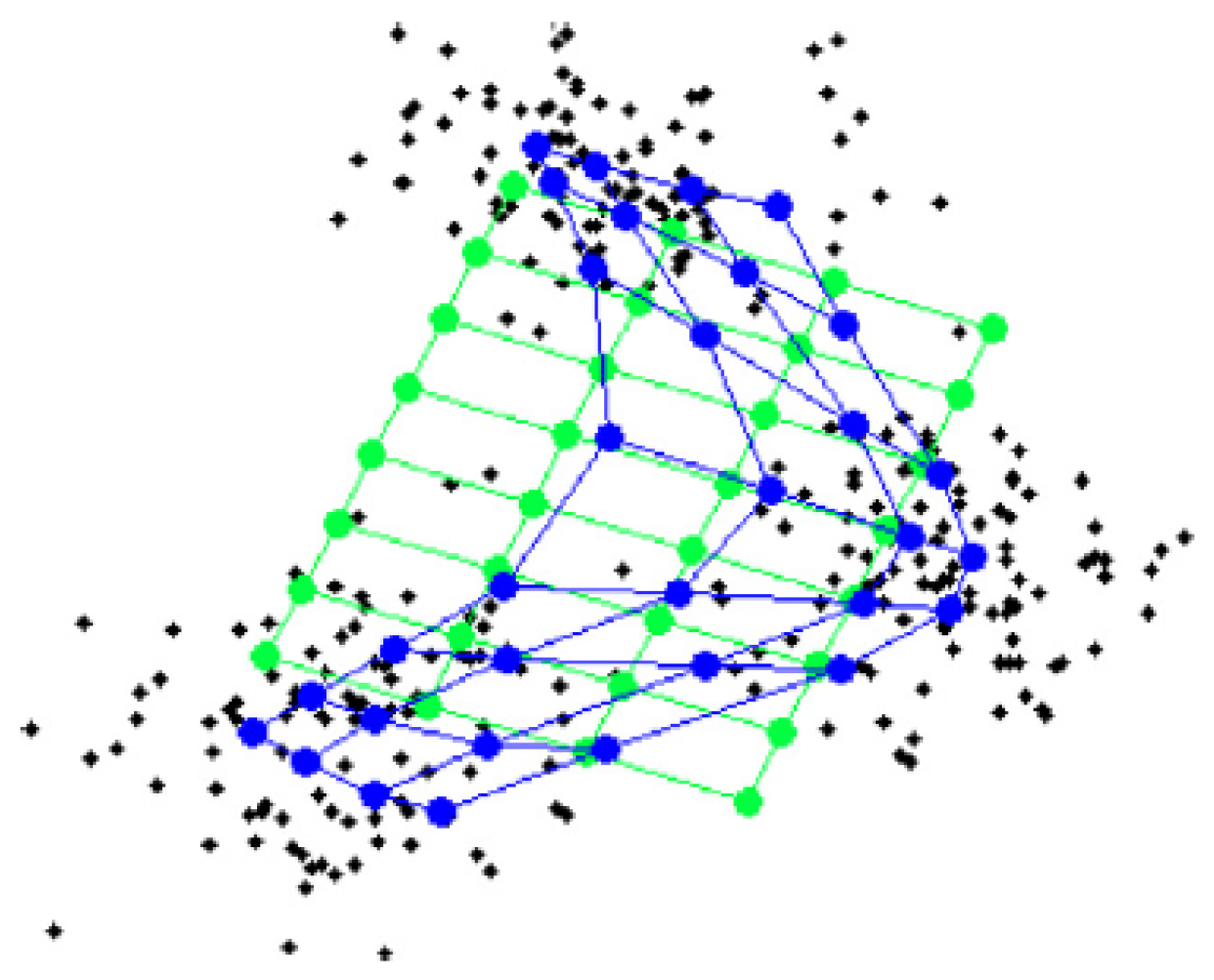
2.3.2. Self-Organizing Map

The self-organizing map (SOM) algorithm [32] from the family of unsupervised neural networks is used for clustering, dimension reduction, and visualization. In this context, ‘unsupervised’ means the relationships in the data are not provided as model input (in terms of input and output data) and the model identifies patterns in the data that are not known beforehand. The SOM algorithm works well with noisy data and can handle large amounts of missingness within the dataset, making it popular for environmental analyses.

The SOM works by placing a mesh of interconnected nodes over a high-dimensional data cloud and, through an iterative process, refining the placement of the nodes to best represent the shape and density of the data, whilst maintaining a connection between neighboring nodes (Figure 2). At each iteration, the Euclidean distance between each node and the nearest data points is measured and the nodes (and their connected neighbors to a lesser extent) are moved towards the nearest data. After the training process (determining the placement of the nodes) is complete, the nodes come to represent the most prevalent patterns that are present in the dataset. In this case, the use of 6 nodes was found to produce the lowest quantization and topographic errors whilst maintaining a manageable number of patterns for interpretation. (Quantization error is a measure of how closely the nodes match the data, and topographic error measures whether similar (nearby) data is represented by neighboring nodes). A final matching step attributes each data item to the nearest node of the trained map based on Euclidean distance in all data dimensions, creating clusters of data that best match each prevalent pattern. In the SOM created here, each dimension of the data represents a year of the study period and, therefore, each resulting cluster contains data points (bores) with similar temporal groundwater patterns over the timeline of the study.

Please refer to [32,33] for further information on the SOM algorithm and to Mangiameli et al. [34,35] for a comparison of SOM and hierarchical clustering methods.

3. Results

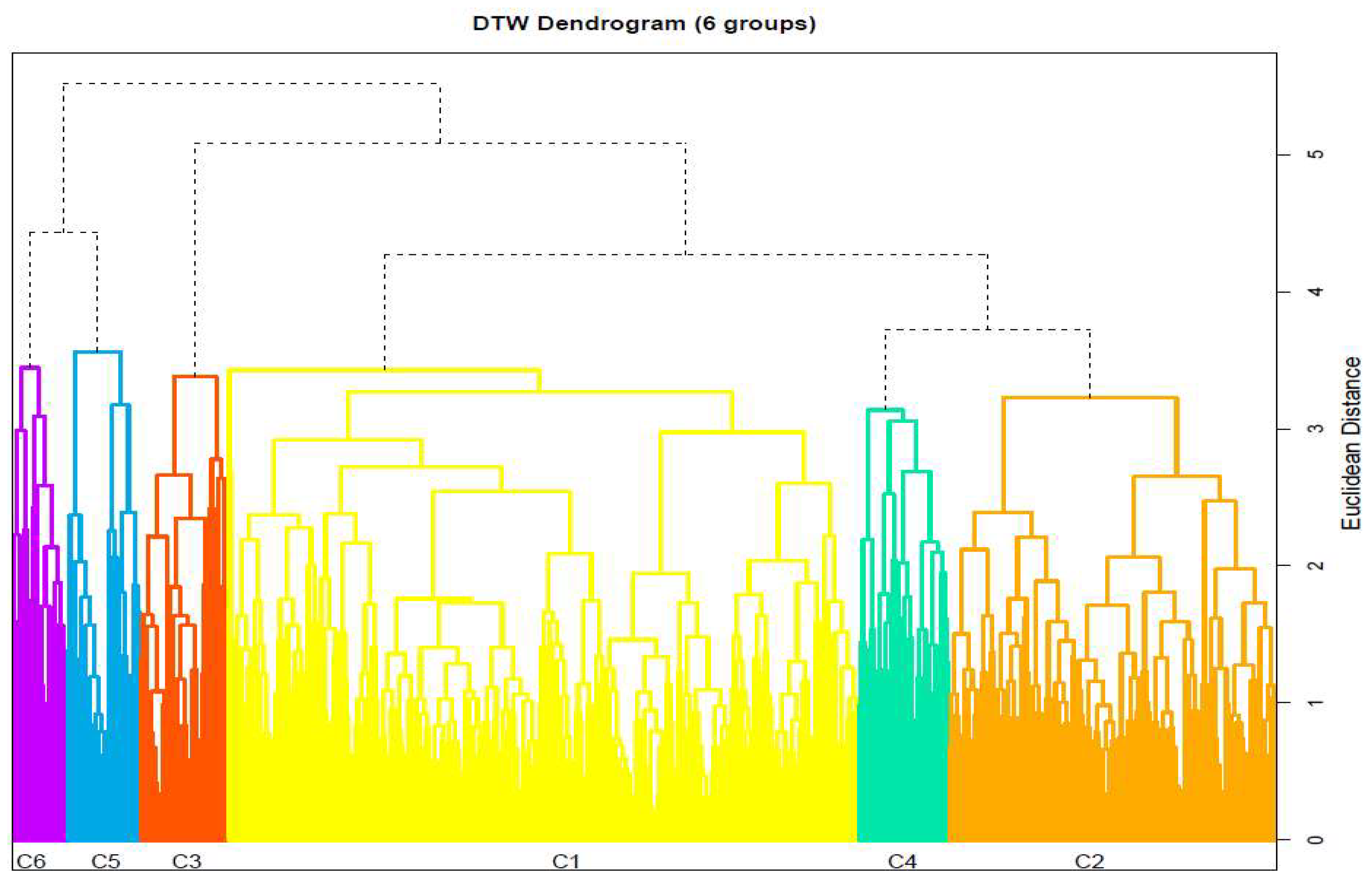
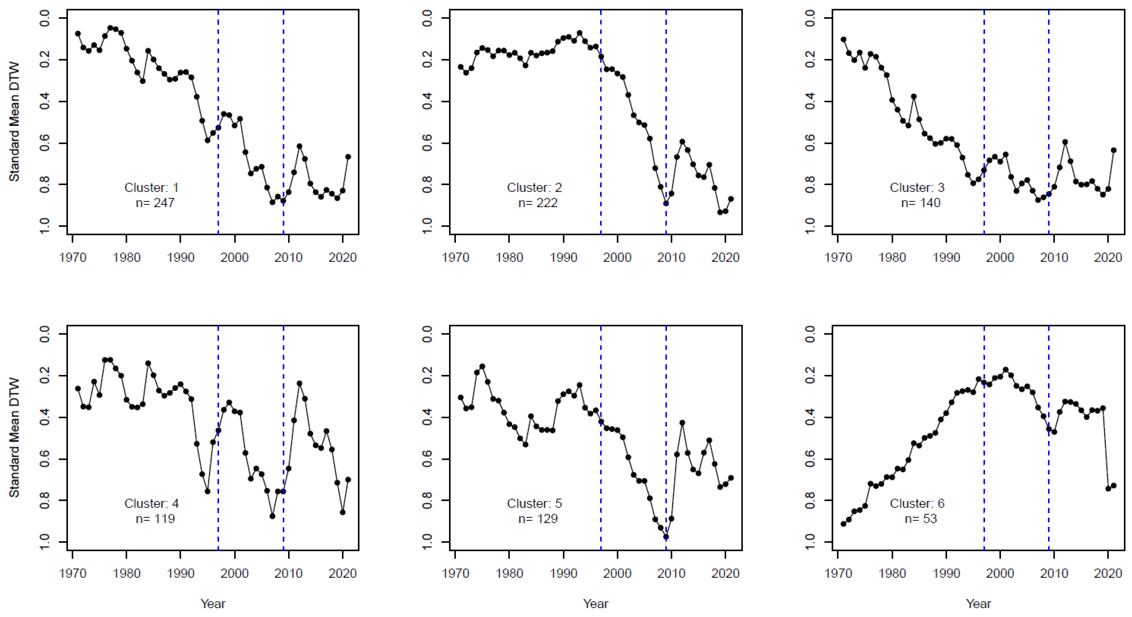
3.1. Clusters of Temporal Patterns of Groundwater Levels

The dendrogram of annual time series of groundwater levels from the 910 study bores is shown in Figure 3. This diagram shows the hierarchical relationship between groundwater bores based on their temporal variability. The most important part to interpreting a dendrogram is the height (Euclidean Distance) at which any two objects are joined together. That is to say, these two objects (groundwater bores in this case) belong to the same group below this distance threshold, but to two different groups above this critical value. It is also important to note that a dendrogram refers to the distance matrix, which implies the original information is lost while computing distance. In addition, a dendrogram itself cannot tell us how many clusters we should use. The number of clusters is usually determined by the distance (although a distance-alone method could lead to an unrealistic number of clusters because it is unlikely for any real-world data to meet the assumption of ultrametric tree inequality), as well as some professional judgements with a bit of trial and error to reflect the physical mechanisms.

Six clusters/groups are chosen from this dendrogram based on these two criteria. The rule to number the clusters from 1 to 6 is based on their temporal variability as shown later in Figure 4, i.e., from a decreasing trend to mixed decreasing/increasing trends and then an increasing trend. A majority of the groundwater bores showed a declining trend, resulting in a large proportion of the observation bores falling within the clusters representing two dominant trends (Clusters 1 and 2).

Figure 4 shows the temporal variations of the annual mean values of the standardized groundwater levels from the six clusters. The vertical dashed lines represent the Millennium Drought period in 1997–2009, a severe and prolonged dry period in southeast Australia. The rainfall, streamflow, groundwater level and storage, wetland, lakes, and their relationships have changed significantly before, during, and after the Millennium Drought [36]. Each cluster displays a unique temporal pattern of groundwater levels as shown in Figure 4:

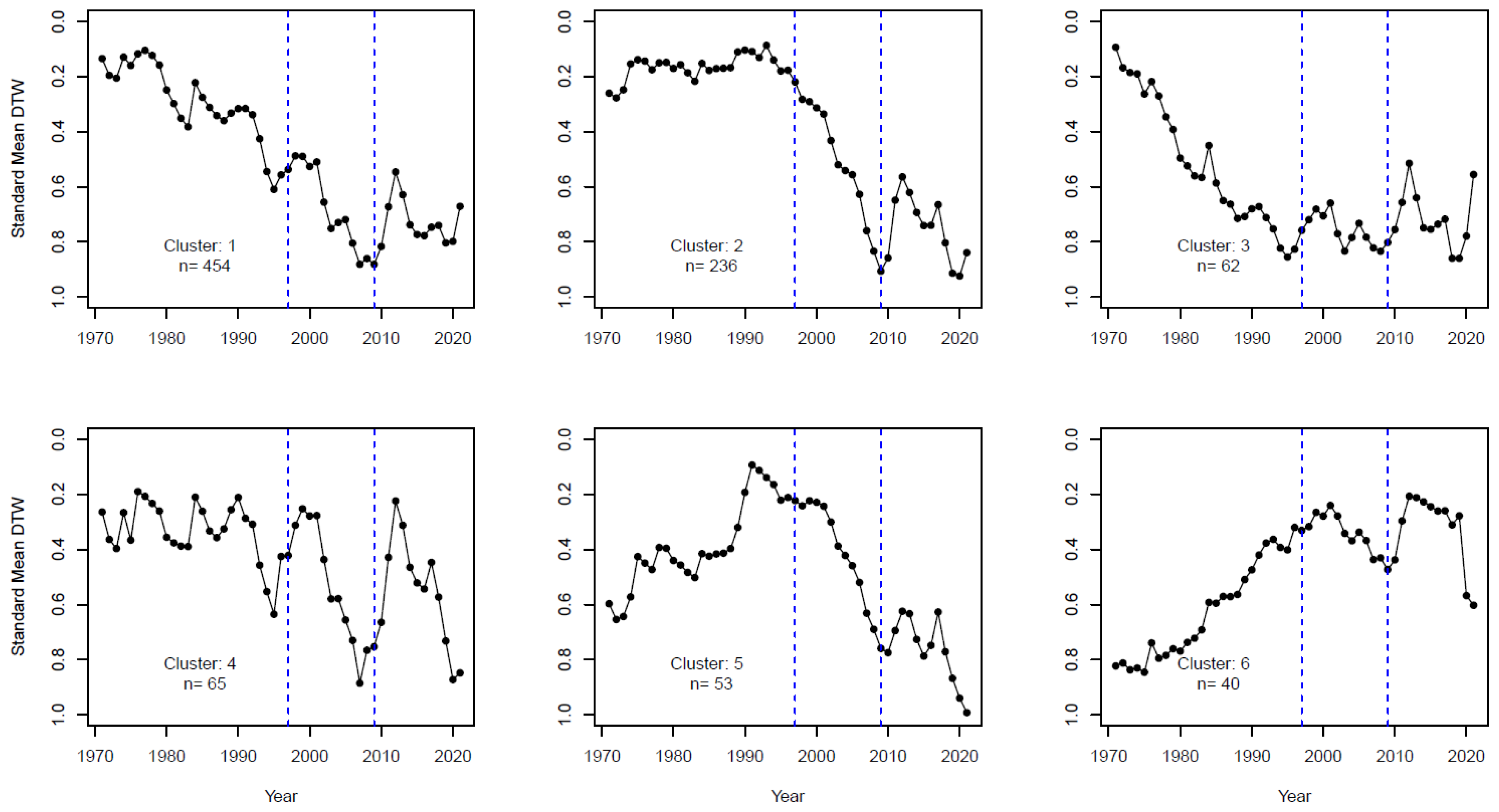
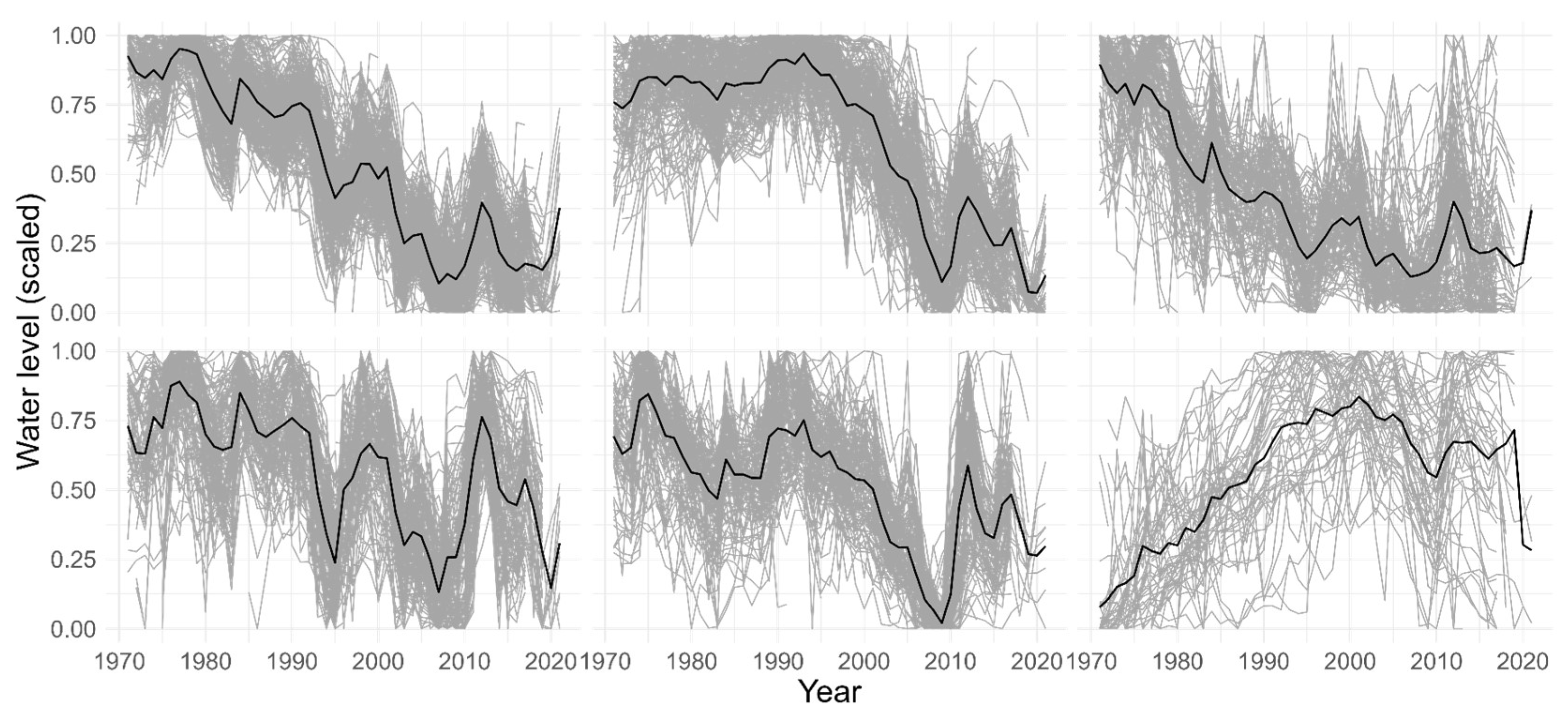
• There are 454 groundwater bores (about 50% of the total 910) in Cluster 1 (C1 in Figure 3), which show a continuous decreasing of groundwater level 1971–2019, i.e., before and during the Millennium Drought (MD) periods. However, the groundwater level is relatively stable after the MD. An increase in groundwater level during the 2011–2012 wet years can also be observed;
• There are 236 groundwater bores (~26%) in Cluster 2, which show a stable groundwater level in 1971–1996 before the MD period but a decreasing trend during and after the MD periods;
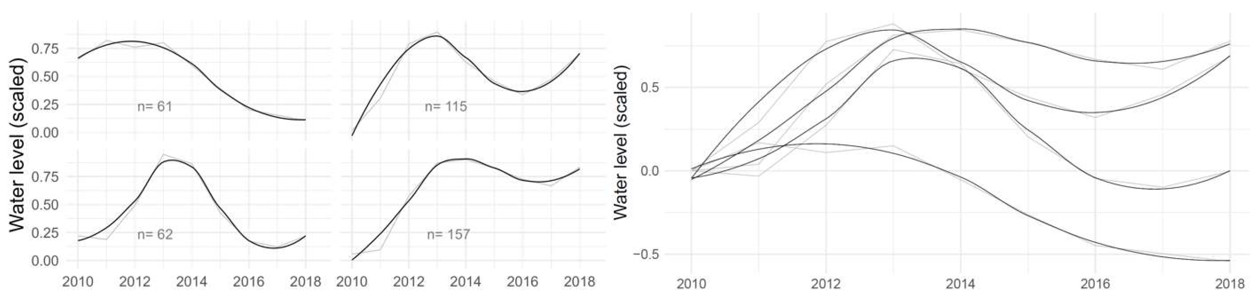
• There are 62 groundwater bores (~7%) in Cluster 3, which show a significant decreasing trend of groundwater level in 1971–1996 before the MD period, but are relatively stable during and after the MD periods;
• There are 65 groundwater bores (~7%) in Cluster 4, which show an overall decreasing trend of groundwater level for the entire study period. However, this time series shows the greatest fluctuation, implying a sensitivity of groundwater level to rainfall anomalies. The 2011–2012 wet years lead to the biggest jump of groundwater level for this cluster;
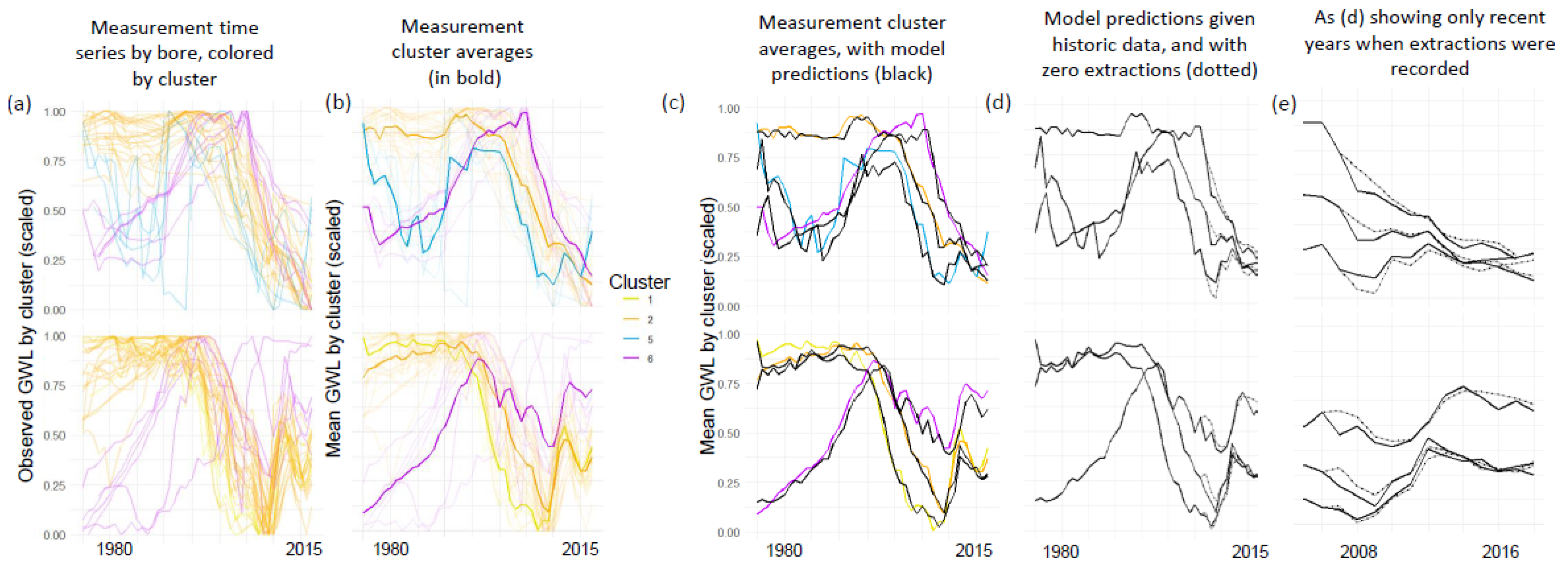
• There are 53 groundwater bores (~6%) in Cluster 5, which show an increasing trend of groundwater level in 1971–1996 before the MD period, but a decreasing trend during and after the MD periods. The increasing trend in 1971–1996 could be the result of human activity, such as irrigation, and the significant decreasing trend during the MD period could be a result of drought events;
• There are 40 groundwater bores (~4%) in Cluster 6, which show a similar increasing trend of groundwater level as seen in Cluster 5 but a relatively stable groundwater level during and after the MD periods. The underlying physical processes could be a mixed impact of human activity and climate change, i.e., the effects of dry climate are offset by human activity.

The cluster results from the self-organizing map are shown in Figure 5. Overall, these results compare well with the hierarchical cluster analysis in Figure 4. The six dominant clusters in groundwater level trends are similarly identified by both techniques. Comparing the clustering results of the hierarchical and SOM methods, the patterns from both methods correspond well for all clusters with the exception of Cluster 5. The number of time series (observation bores) that best match each pattern differs between methods, with about half of the time series that are attributed to Cluster 1 with the hierarchical clustering method spread between Clusters 3, 4, and 5 with the SOM. The number of time series in Clusters 2 and 6 are almost the same for both clustering methods, indicating a clear separation of these bores in which groundwater levels were not declining prior to the MD.

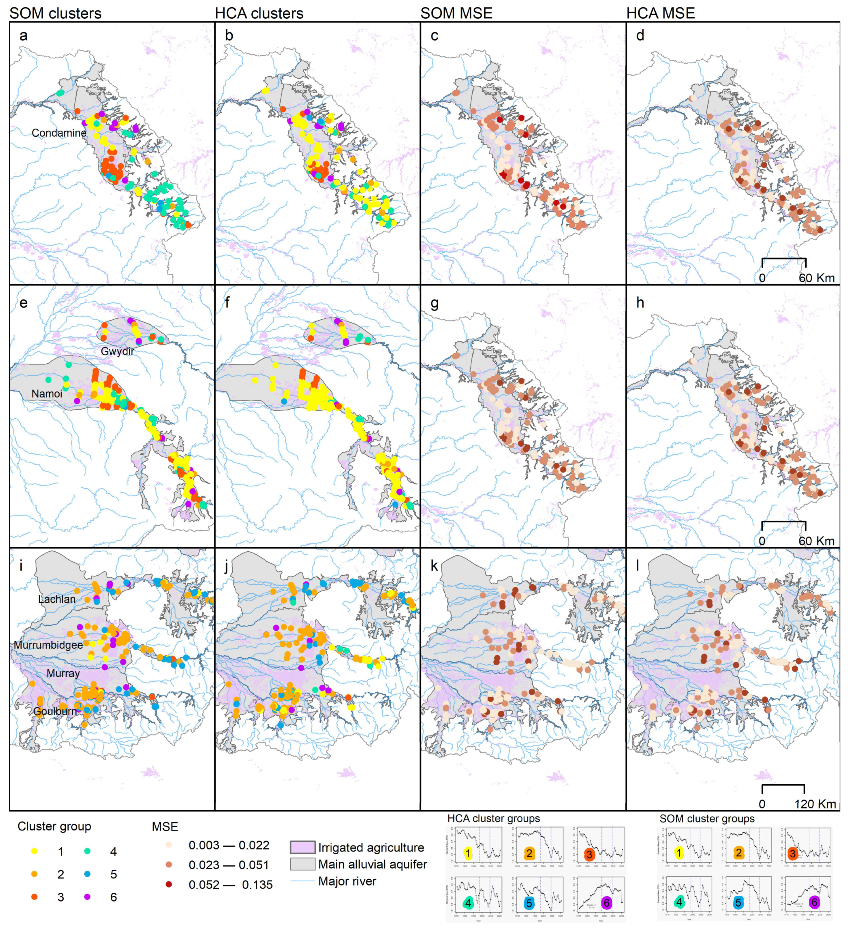
3.2. Spatial Distributions of Groundwater Level Temporal Patterns

Figure 6 shows the spatial distributions of the temporal patterns of groundwater levels obtained from the hierarchical clustering analysis (HCA) and SOM. Bores are colored by cluster as indicated in the legend. It can be seen that the region shown in the upper row (Condamine) contains a mixture of all patterns; the middle row (Namoi, Gwydir) has mostly yellow and red bores (relatively constant decline before and during drought, evening out post-drought), with some turquoise—the turquoise pattern is similar to the yellow and red, but shows better recovery between drawdown events; and the region in the lower row (Lachlan, Murrumbidgee, Murray, Goulburn) is dominated by orange (stable pre-drought followed by a steep decline during the Millennium Drought) with some blues (steep decline but more recovery) and purples (increasing before and immediately after the drought).

In terms of the mean square error (MSE), both clustering techniques show similar numerical performance. Two areas of discrepancy arise in the upper Condamine Tributaries (Figure 6a vs. Figure 6b) and the Mid-Murrumbidgee (Figure 6i vs. Figure 6j). In the former, bores are identified with Cluster 4 (SOM) and Cluster 1 (HCA). Both clusters are similar with the cluster identified by the SOM showing a higher range in the representative times series. For Mid-Murrumbidgee, the clustered patterns are similar and only differ in the stable trend prior to the pronounced declining trend, e.g., Cluster 5 (SOM) vs. Cluster 2 (HCA).

The geographic distributions of the hierarchical clustering results are generally consistent with those of the SOM clustering results (Figure 6). However, one of the significant differences is that Cluster 1 includes 454 out of 910 of groundwater bores (about 50%) from the hierarchical clustering (Figure 4), but only 247 out of 910 bores (27%) based on the SOM clustering (Figure 5), indicating that Cluster 1 has a wider spatial distribution for the hierarchical clustering results (Figure 6) due to the attribution of more bores to Clusters 3, 4, and 5 with the SOM, as discussed in Section 3.1.

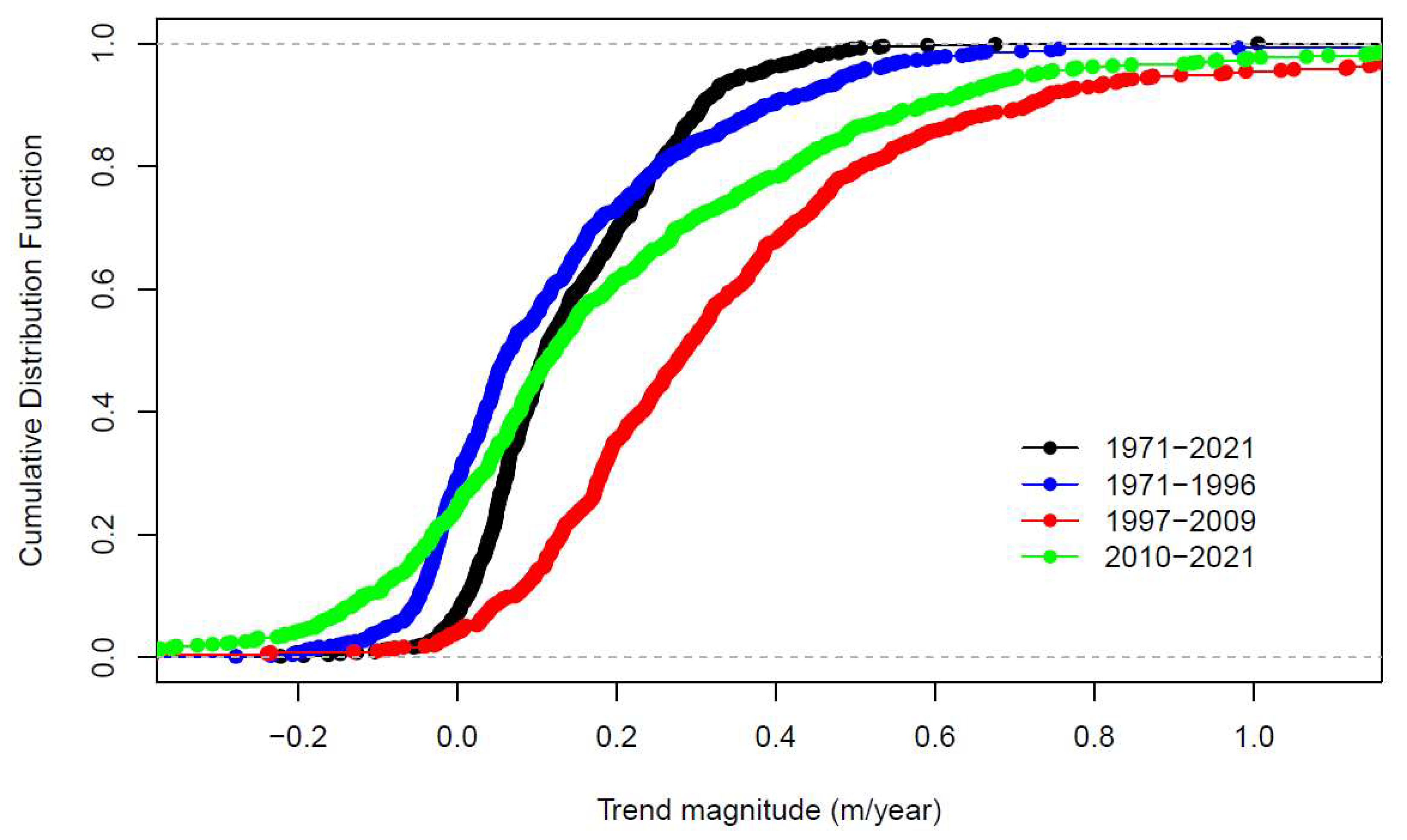
3.3. Impacts of the Millennium Drought on Groundwater Level Trends and Clustering Results

As this data set contains groundwater level measurements from before, during, and after the Millennium Drought, further analysis is conducted here to determine whether areas with similar groundwater patterns before and during the drought continued to behave similarly after the drought; that is, whether the drought imposed diverse outcomes on regions with heretofore similar groundwater patterns.

For this analysis, the time series are split into three periods corresponding to before (1971–1996), during (1997–2009), and after (2010–2021) the Millennium Drought [20]. However, we cannot use all 910 bores for this analysis, as the data filtering criterion (at least two records per year for at least 40 years during the 51-year study period) are applied to the entire study period 1971–2021. It is not suitable for three sub-period trend detections, because it can lead to a very small sample size for one period. For example, all 11 missing years for a specific bore may be located at the post-drought 2010–2021 period, resulting in only one data point available for the groundwater level time series at this bore and, accordingly, a meaningless trend magnitude. A sub-set of 661 of the 910 bores is selected by requiring at least 70% of data points of groundwater level time series at each of the three time periods, i.e., before, during, and after the MD.

Figure 7 shows the cumulative distribution function of trend magnitude of groundwater levels in these three periods. The magnitude value indicates the rate of change in the groundwater level over time. Because it is based on depth to standing water level measurements, a positive magnitude indicates a decline in groundwater level, i.e., groundwater level becoming deeper with time.

Over this sub-set of bores, it is evident from Figure 7 that the trend magnitudes are the largest (indicating a steeper decline in groundwater level) during the Millennium Drought period due to the dry climate (Figure 7 and

Table 1. Number of bores with trend significance in four study periods (α = 0.05 significance level).

Study Period	Sig Rise	Rise	Decline	Sig Decline
1971–2021	33	13	31	584
1971–1996	97	95	85	384
1997–2009	11	17	71	562
2010–2021	33	149	332	147

). In contrast, trend magnitudes before the MD period are the smallest because of a wetter climate, and the magnitudes after the MD period generally fall into the middle except for the negative trend magnitudes. The negative trend magnitudes after the MD period at 20–25% of groundwater bore locations imply the recovery of groundwater levels is observed from the dry period to wet climate conditions. The remaining 75–80% of the bores still show a decrease in groundwater levels, but their magnitudes and significance are smaller than those observed during the MD period (Figure 7 and Table 1).

The back-to-normal rainfall after the MD may provide insightful information into recent regional groundwater behavior. Observation bores that were behaving similarly before and during the drought may have different post-drought responses. To investigate this, a new SOM is created in which the set of time series are first clustered based on before- and during-drought patterns, and these clusters are then refined by post-drought information. The three main patterns identified in the data before and during the drought by this SOM are shown in Figure 8. Note that there are now three main patterns identified rather than the six identified in the previous section, as the post-drought period is not being considered here. The three main patterns are characterized by groundwater levels remaining steady before the drought followed by a swift decline during the drought (on the left, roughly corresponding to data from Cluster 2 and some from Clusters 4 and 5 in Figure 5), a constant decline before and during the MD (center, corresponding mostly to Clusters 1 and 3 in Figure 5), and a general increase in groundwater levels until the drought followed by a decline (on the right, corresponding mostly to Cluster 6 in Figure 5).

These groundwater level patterns before and during the drought can now be refined by information from after the drought. For example, the 401 bores from the first cluster of Figure 8 (with groundwater levels steady before the drought and declining during the drought) are further clustered in Figure 9 based on post-drought measurements. Four patterns of post-drought behavior are observed, all of which have some degree of increased groundwater level immediately following the drought (Figure 9). After this initial post-drought increase, the behavior diversifies into further increase, steadying, or declining. Figure 9 shows the four patterns with an aligned origin for comparison purposes.

4. Discussion

4.1. Implications for Groundwater Management

Temporal groundwater level patterns vary abruptly across space in this region, implying the complexity of the groundwater system. For example, two groundwater bores in close proximity could exhibit different temporal patterns due to different hydrogeological settings. This presents a challenge for regional groundwater planning and management, as different bores in the same location may indicate different temporal variability. On the other hand, groundwater bores in different spatial resource units could show similar temporal patterns. It has been shown that the six predominant temporal patterns identified in this study transcend SDL resource unit boundaries. Figure 10 depicts these six patterns along with all of the bore time series that match each pattern, though the bores in each cluster may be located in any of the resource units. Considering the 900+ groundwater time series in this region as members of six clusters could lead to pattern-centric management considerations.

Knowledge gained from the clustering analysis about the six predominant groundwater patterns found in this river system could allow for information to be shared across the region and produce a refinement of groundwater level estimations within each resource unit. This would enable the use of a method similar to the clustering/deep learning framework used in [37] to be used for groundwater level predictions within the MDB, which was shown to be useful at estimating groundwater levels in locations where few historical measurements exist through the leveraging of information from data-rich locations with similar patterns.

The findings of this study can be used to inform sub-regional resource unit policy and planning decisions to better manage drought and climate change in the future, including innovative interventions such as managed aquifer recharge and conjunctive water-use management.

4.2. Method Comparison

Overall, the two popular clustering methods used in this study, hierarchical clustering analysis and self-organizing maps, produced six similar predominant temporal patterns from a dataset of 910 observation bore time series, implying robust identification of the main temporal patterns of groundwater levels in the study region.

A difference arose in the number of time series (observation bores) which were allocated to each cluster; however, a geographical analysis indicated that this was the result of time series within specific areas being attributed to closely related patterns. The number of time series representing bores with steady or increasing groundwater levels before the Millenium Drought are almost the same for both clustering methods. A potential caveat of the two approaches used in this study is that the spatial proximity of bores was not considered during the clustering process, though this was a conscious decision as the subsurface conditions, such as connectivity of the aquifers, are not known. How to improve on this is complicated in this study domain because two bores that are close to each other in space could access different aquifers with significantly different groundwater depths, such as one from a shallow aquifer and another from a deep aquifer in the same location.

The SOM neural network clustering methodology has been demonstrated to be superior to the traditional hierarchical clustering method by [34]. However, our results indicated that the two methods showed similar results and confirm the likelihood that the prevalent patterns have been identified. Furthermore, the combination of the two methods might lead to a more reliable result [35], but it needs further investigation to make a solid conclusion.

4.3. Potential for Attribution of Drivers of Groundwater Level Changes

As groundwater level patterns have been found to differ within each resource unit and yet maintain similarities across the resource units, a causal attribution framework could be developed to determine the main influences on groundwater level changes in each region. For example, groundwater extractions may be strongly influencing groundwater depletion in some locations, whereas other areas may be more affected by changes in rainfall and PET. Similarly, groundwater levels in some areas may be more affected by the changing nature of surface water/groundwater connectivity. This type of attribution or sensitivity analysis would involve representing the system with a model that can simulate changes in groundwater levels given certain climate and anthropogenic conditions, as in [38,39].The model could then be probed to determine which driving factors are having the greatest impact on groundwater levels, using a mixture of visual and computational methods. It is possible to investigate these attributions temporally as well as spatially to determine if the main factors contributing to altered groundwater levels have transformed over time.

An example attribution analysis is shown here for two resource units. A neural network model is trained to represent the groundwater level response at each measurement bore (i.e., change in groundwater level) to a set of conditions represented by predictor variables (current rainfall, antecedent rainfall in previous 3 years, previous groundwater level, PET, and groundwater extractions). The cluster membership of each groundwater bore is also included. All variables besides cluster membership are annual mean measurements. Though multiple groundwater measurement bores are located within each resource unit, the observed rainfall, evapotranspiration, and extraction data are at the resource unit level (i.e., one value per resource unit). The predictor variables are scaled into the range [0,1] by resource unit to facilitate comparisons between systems at dissimilar scales. Groundwater level measurements have been scaled to the range [0,1] by bore. A feed-forward neural network (or multi-layer perceptron, MLP) is used to model the changes in groundwater levels for the set of predictors. Model settings (hyperparameters) have not been optimized in this preliminary analysis.

Results of this preliminary attribution analysis are outlined in Figure 11. Figure 11a shows the scaled groundwater measurements for the bores in the two sample resource units. For visualization purposes, these observations are colored by the cluster pattern from Figure 6 that they best match, with the cluster average overlaid in bold on Figure 11b. Each resource unit has a different set of patterns represented within it, and not all patterns are found in all resource units. In Figure 11c, the mean modeled groundwater levels are shown in black over the colored mean measurements for each cluster. There are as many predictions produced for each resource unit as there are predominant groundwater patterns within it. It can be seen that this is beneficial compared with producing a single annual prediction for each resource unit, which would miss much of the inter-cluster measurement variation.

The next step in the causal attribution analysis is to interrogate the models to determine how each predictor variable influences annual changes in groundwater levels. Counterfactual scenarios or perturbations of input variables could be explored in which the effect of certain predictors on the modeled results are examined. For example, Figure 11d provides a visualization of the counterfactual scenario in which no extractions occurred in these sample resource units. This is the result of re-running the trained model with a new set of data in which groundwater use (extraction data) is artificially set to zero. The dashed line shows the estimation of groundwater levels without extractions (see Figure 11e for a zoomed-in version). The effect of groundwater extractions differs by cluster even within the same resource unit. This may be due to some bores receiving an influx of water if the extracted groundwater is then used for local irrigation.

Understanding the factors driving changes in the various groundwater level patterns may help to focus specific efforts for maintaining sustainable groundwater resources. A full analysis of all resource units or additional possible drivers of change is outside the scope of the current project and will be considered for future work.

4.4. Data Quality

A consideration of data quality is always critical for analyses that use data-driven models, and in the context of this study data quality issues include but are not limited to the following: (a) The groundwater level observations are generally acceptable, but obvious errors and outliers exist. Suspicious observations are very common for groundwater level measurements [40], which could come from several reasons [10,40] such as a simple record error, failure of a data log, or an unforeseen biophysical and hydrological process (e.g., a flood event, nearby pump testing, or sudden groundwater extraction). These may provide valuable insights about groundwater dynamics, but they were not further investigated and were removed for this study [10]; (b) At least two observations per year were required to produce an annual time series of groundwater level [10]. This is based on a sampling strategy that could capture the highest and lowest groundwater levels in a given year at a specific location, but this assumption cannot be verified without further investigations; (c) SILO rainfall and PET climate data based on high-quality meteorological stations have been widely used for various engineering and scientific applications with acceptable accuracy. However, a recent study showed that SILO could also generate larger than expected uncertainty, especially in regions with limited weather stations [27]; (d) The biggest challenge might come from the groundwater extraction data for the attribution analysis due to the nonexistence of reliable long-term data. For example, we could only collect groundwater extraction information since 2006, and there is no doubt that there are some unmetered extraction volumes. These limitations of groundwater extraction data may present a challenge for a full-scale comprehensive attribution analysis.

5. Conclusions

Two popular clustering methods, hierarchical clustering analysis and the self-organizing map, are used in this study to investigate the temporal patterns of groundwater levels from a dataset with 910 observation bores. Six dominant patterns (and associated clusters of bores) were found using both methods. These established patterns provide additional temporal and spatial granularity, building on a previous study of historical groundwater levels trends (1971–2021) in the Murray–Darling Basin [10]. The spatial distribution of the temporal patterns shows that different areas had different responses to severe drought and to post-drought recharge and recovery. This provides important information to guide management and planning decisions at finer spatial scales.

Overall, the two clustering methods produced similar patterns with comparable numerical performance, indicating the robustness of the six dominant patterns that have been identified. A difference arose in the number of time series which were allocated to each cluster; however, a geographical analysis indicated that this was the result of time series within specific areas being attributed to closely related patterns.

The Millennium Drought from 1997 to 2009 had a clear impact on groundwater level temporal variability and trends. The trend magnitudes of groundwater levels were the largest (indicating a steeper decline in groundwater level) during the drought period due to the dry climate. In contrast, trend magnitudes before the drought period are the smallest because of a wetter climate.

Accessing spatially and temporally comprehensive data on groundwater use will largely determine the quality of any causal inference of groundwater trends under anthropogenic conditions. An example attribution analysis was shown here for two resource units using a neural network model. In future work, this model will be improved and expanded to identify drivers of groundwater level change for each of the dominant patterns in the basin.

References

1. Elshall, A.S.; Arik, A.D.; El-Kadi, A.I.; Pierce, S.; Ye, M.; Burnett, K.M.; Wada, C.A.; Bremer, L.L.; Chun, G. Groundwater sustainability: A review of the interactions between science and policy. Environ. Res. Lett. 2020, 15, 093004. [Google Scholar] [CrossRef]
2. Rojas, R.; Gonzalez, D.; Fu, G. Resilience, stress and sustainability of alluvial aquifers in the Murray-Darling Basin, Australia: Opportunities for groundwater management. J. Hydrol. Reg. Stud. 2023, 47, 101419. [Google Scholar] [CrossRef]
3. Anderson, M.P. Groundwater Research and Management: New Directions and Re-invention. In Groundwater as a Key for Adaptation to Changing Climate and Society; Taniguchi, M., Hiyama, T., Eds.; Springer: Tokyo, Japan, 2014; pp. 1–15. [Google Scholar]
4. de Graaf, I.E.M.; Gleeson, T.; van Beek, L.P.H.; Sutanudjaja, E.H.; Bierkens, M.F.P. Environmental flow limits to global groundwater pumping. Nature 2019, 574, 90–94. [Google Scholar] [CrossRef] [PubMed]
5. Martinsen, G.; Bessiere, H.; Caballero, Y.; Koch, J.; Collados-Lara, A.J.; Mansour, M.; Sallasmaa, O.; Pulido-Velazquez, D.; Williams, N.H.; Zaadnoordijk, W.J.; et al. Developing a pan-European high-resolution groundwater recharge map—Combining satellite data and national survey data using machine learning. Sci. Total Environ. 2022, 822, 153464. [Google Scholar] [CrossRef] [PubMed]
6. Milman, A.; MacDonald, A. Focus on interactions between science-policy in groundwater systems. Environ. Res. Lett. 2020, 15, 090201. [Google Scholar] [CrossRef]
7. Fu, G.; Schmid, W.; Castellazzi, P. Understanding the Spatial Variability of the Relationship between InSAR-Derived Deformation and Groundwater Level Using Machine Learning. Geosciences 2023, 13, 133. [Google Scholar] [CrossRef]
8. Lasagna, M.; Mancini, S.; De Luca, D.A. Groundwater hydrodynamic behaviours based on water table levels to identify natural and anthropic controlling factors in the Piedmont Plain (Italy). Sci. Total Environ. 2020, 716, 137051. [Google Scholar] [CrossRef]
9. Tillman, F.D.; Leake, S.A. Trends in groundwater levels in wells in the active management areas of Arizona, USA. Hydrogeol. J. 2010, 18, 1515–1524. [Google Scholar] [CrossRef]
10. Fu, G.B.; Rojas, R.; Gonzalez, D. Trends in Groundwater Levels in Alluvial Aquifers of the Murray-Darling Basin and Their Attributions. Water 2022, 14, 1808. [Google Scholar] [CrossRef]
11. Konikow, L.F.; Kendy, E. Groundwater depletion: A global problem. Hydrogeol. J. 2005, 13, 317–320. [Google Scholar] [CrossRef]
12. Wada, Y.; van Beek, L.P.H.; van Kempen, C.M.; Reckman, J.W.T.M.; Vasak, S.; Bierkens, M.F.P. Global depletion of groundwater resources. Geophys. Res. Lett. 2010, 37, L20402. [Google Scholar] [CrossRef]
13. Famiglietti, J.S. The global groundwater crisis. Nat. Clim. Chang. 2014, 4, 945–948. [Google Scholar] [CrossRef]
14. Bennett, G.; Van Camp, M.; Shemsanga, C.; Kervyn, M.; Walraevens, K. Assessment of spatial and temporal variability of groundwater level in the aquifer system on the flanks of Mount Meru, Northern Tanzania. J. Hydrol. Reg. Stud. 2022, 44, 101212. [Google Scholar] [CrossRef]
15. Yin, J.N.; Medellin-Azuara, J.; Escriva-Bou, A. Hierarchical clustering and regional drought assessment of groundwater levels in heavily drafted aquifers. Hydrol. Res. 2022, 53, 1031–1046. [Google Scholar] [CrossRef]
16. Marchant, B.P.; Cuba, D.; Brauns, B.; Bloomfield, J.P. Temporal interpolation of groundwater level hydrographs for regional drought analysis using mixed models. Hydrogeol. J. 2022, 30, 1801–1817. [Google Scholar] [CrossRef]
17. Naranjo-Fernández, N.; Guardiola-Albert, C.; Aguilera, H.; Serrano-Hidalgo, C.; Montero-González, E. Clustering Groundwater Level Time Series of the Exploited Almonte-Marismas Aquifer in Southwest Spain. Water 2020, 12, 1063. [Google Scholar] [CrossRef]
18. Wu, R.S.; Hussain, F.; Lin, Y.C.; Yeh, Z.Y.; Yu, K.C. Characterization of Regional Groundwater System Based on Aquifer Response to Recharge-Discharge Phenomenon and Hierarchical Clustering Analysis. Water 2021, 13, 2535. [Google Scholar] [CrossRef]
19. Clark, S.R. Unravelling groundwater time series patterns: Visual analytics-aided deep learning in the Namoi region of Australia. Environ. Model. Softw. 2022, 149, 105295. [Google Scholar] [CrossRef]
20. Fu, G.; Chiew, F.H.S.; Post, D.A. Trends and variability of rainfall characteristics influencing annual streamflow: A case study of southeast Australia. Int. J. Climatol. 2023, 43, 1407–1430. [Google Scholar] [CrossRef]
21. Leblanc, M.; Tweed, S.; Van Dijk, A.; Timbal, B. A review of historic and future hydrological changes in the Murray-Darling Basin. Glob. Planet. Chang. 2012, 80–81, 226–246. [Google Scholar] [CrossRef]
22. Qureshi, M.E.; Whitten, S.M. Regional impact of climate variability and adaptation options in the southern Murray–Darling Basin, Australia. Water Resour. Econ. 2014, 5, 67–84. [Google Scholar] [CrossRef]
23. Yu, J.J.; Fu, G.B.; Cai, W.J.; Cowan, T. Impacts of precipitation and temperature changes on annual streamflow in the Murray-Darling Basin. Water Int. 2010, 35, 313–323. [Google Scholar] [CrossRef]
24. Crosbie, R.S.; McCallum, J.L.; Walker, G.R.; Chiew, F.H.S. Modelling climate-change impacts on groundwater recharge in the Murray-Darling Basin, Australia. Hydrogeol. J. 2010, 18, 1639–1656. [Google Scholar] [CrossRef]
25. BOM. National Groundwater Information System. Available online: http://www.bom.gov.au/water/groundwater/ngis/ (accessed on 6 January 2021).
26. Jeffrey, S.J.; Carter, J.O.; Moodie, K.B.; Beswick, A.R. Using spatial interpolation to construct a comprehensive archive of Australian climate data. Environ. Model. Softw. 2001, 16, 309–330. [Google Scholar] [CrossRef]
27. Fu, G.B.; Barron, O.; Charles, S.P.; Donn, M.J.; Van Niel, T.G.; Hodgson, G. Uncertainty of Gridded Precipitation at Local and Continent Scales: A Direct Comparison of Rainfall from SILO and AWAP in Australia. Asia-Pac. J. Atmos. Sci. 2022, 58, 471–488. [Google Scholar] [CrossRef]
28. Walker, G.; Barnett, S.; Richardson, S. Developing a Coordinated Groundwater Management Plan for the Interstate Murray-Darling Basin. In Sustainable Groundwater Management: A Comparative Analysis of French and Australian Policies and Implications to Other Countries; Rinaudo, J.-D., Holley, C., Barnett, S., Montginoul, M., Eds.; Springer International Publishing: Cham, Switzerland, 2020; pp. 143–161. [Google Scholar]
29. Stewardson, M.J.; Walker, G.; Coleman, M. Chapter 3—Hydrology of the Murray-Darling Basin. In Murray-Darling Basin, Australia; Hart, B.T., Bond, N.R., Byron, N., Pollino, C.A., Stewardson, M.J., Eds.; Elsevier: Amsterdam, The Netherlands, 2021; Volume 1, pp. 47–73. [Google Scholar]
30. MDBA. Transition Period Water Take Report 2018–19; MDBA Publication No: 38/20; Murray-Darling Basin Authority: Canberra, Australia, 2020. [Google Scholar]
31. Nielsen, F. Hierarchical Clustering. In Introduction to HPC with MPI for Data Science; Nielsen, F., Ed.; Springer International Publishing: Cham, Switzerland, 2016; pp. 195–211. [Google Scholar]
32. Kohonen, T. The self-organizing map. Proc. IEEE 1990, 78, 1464–1480. [Google Scholar] [CrossRef]
33. Clark, S.; Sisson, S.A.; Sharma, A. Tools for enhancing the application of self-organizing maps in water resources research and engineering. Adv. Water Resour. 2020, 143, 103676. [Google Scholar] [CrossRef]
34. Mangiameli, P.; Chen, S.K.; West, D. A comparison of SOM neural network and hierarchical clustering methods. Eur. J. Oper. Res. 1996, 93, 402–417. [Google Scholar] [CrossRef]
35. Shahid, N. Comparison of hierarchical clustering and neural network clustering: An analysis on precision dominance. Sci. Rep. 2023, 13, 5661. [Google Scholar] [CrossRef]
36. Fu, G.B.; Chiew, F.H.; Zheng, H.X.; Robertson, D.E.; Potter, N.J.; Teng, J.; Post, D.A.; Charles, S.P.; Zhang, L. Statistical analysis of attributions of climatic characteristics to nonstationary rainfall-streamflow relationship. J. Hydrol. 2021, 603, 127017. [Google Scholar] [CrossRef]
37. Clark, S.R.; Pagendam, D.; Ryan, L. Forecasting Multiple Groundwater Time Series with Local and Global Deep Learning Networks. Int. J. Environ. Res. Public Health 2022, 19, 5091. [Google Scholar] [CrossRef]
38. Amaranto, A.; Pianosi, F.; Solomatine, D.; Corzo, G.; Muñoz-Arriola, F. Sensitivity analysis of data-driven groundwater forecasts to hydroclimatic controls in irrigated croplands. J. Hydrol. 2020, 587, 124957. [Google Scholar] [CrossRef]
39. Wunsch, A.; Liesch, T.; Broda, S. Deep learning shows declining groundwater levels in Germany until 2100 due to climate change. Nat. Commun. 2022, 13, 1221. [Google Scholar] [CrossRef]
40. Peterson, T.J.; Western, A.W.; Cheng, X. The good, the bad and the outliers: Automated detection of errors and outliers from groundwater hydrographs. Hydrogeol. J. 2018, 26, 371–380. [Google Scholar] [CrossRef]
Figure 1. Distribution of observation bores used in this study across the resource units comprising the main alluvial aquifer systems in the Murray–Darling Basin (modified from Rojas et al., 2023 [2]).
Sustainability 15 16295 g001
Figure 2. SOM schematic: a mesh of interconnected nodes (green) is placed over a data set (black dots, 2D toy data for the purpose of visualization); the mesh is then trained (bent and stretched) to better match the data distribution, resulting in the final map configuration (blue); data items are matched to their nearest map node to create clusters of similar items (modified from Clark et al., 2020 [33]).
Sustainability 15 16295 g002
Figure 3. Dendrogram of groundwater levels from 910 bores, separated into six groups/clusters with the hierarchical clustering algorithm. The labels C1, C2, etc., refer to ‘Cluster 1′, Cluster 2′, etc.
Sustainability 15 16295 g003
Figure 4. Time series of annual mean standardized groundwater level (depth to water level, DTW) from six clusters based on hierarchical cluster analysis. The vertical blue dashed lines represent the Millennium Drought period from 1997–2009.
Sustainability 15 16295 g004
Figure 5. Clusters of groundwater level time series determined with the self-organizing map algorithm.
Sustainability 15 16295 g005
Figure 6. Spatial distributions of cluster patterns of groundwater level temporal variability from the self-organizing map (SOM, a,e,i) and the hierarchical cluster analysis (HCA, b,f,j) clustering techniques with mean square error (MSE) shown for SOM (c,g,k) and HCA (d,h,l). The patterns that are predominantly found in each geographical area can be seen—in the Condamine region (ad), all patterns are represented; in the Gwydir/Namoi region (eh), Clusters 1, 3, and 4 are most commonly found; and in the Lachlan, Murrumbidgee, Murray, and Goulburn region (il), Clusters 2, 5, and 6 dominate.
Sustainability 15 16295 g006
Figure 7. Slopes of groundwater level time series separated into three segments: before MD 1971–1996 (dark blue), MD 1997–2009 (red), and after MD 2010–2017 green), as well as the entire study period (black). Positive slopes mean the groundwater level is decreasing over time.
Sustainability 15 16295 g007
Figure 8. Three main patterns in groundwater levels before and during the Millennium Drought (1971–2009) as found by the SOM (grey) with overlayed smoothers (black). The number of time series that match each pattern is denoted in the lower left of each plot.
Sustainability 15 16295 g008
Figure 9. Prevalent patterns of post-drought behavior (2010–2018) in groundwater time series that were steady before the Millennium Drought but declined during the drought (first cluster of Figure 8) are shown in grey with smoothers overlayed in black. The left panel shows the four patterns of post-drought behavior found in these bores, all of which exhibit some recovery in groundwater level immediately after the drought (2010–2012) followed by a diversity of behaviors. On the right panel, the origins of these patterns are aligned for comparison of the potential groundwater level paths for these bores that had similar behavior before and during the drought.
Sustainability 15 16295 g009
Figure 10. Measurements from all study bores plotted in their matching SOM cluster (grey lines) with the SOM cluster pattern in black. This illustrates the similarities of time series patterns in each cluster that transcend SDL resource unit boundaries.
Sustainability 15 16295 g010
Figure 11. A sample attribution analysis on two resource units, showing the following: (a) measured groundwater level historic data (colored by cluster); (b) cluster mean measurements in bold; (c) modeled annual groundwater levels for each cluster (black) shown over cluster mean measurements (colored); (d) modeled annual groundwater levels for each cluster (black) and the hypothetical scenario if no extractions had occurred (dotted); (e) as above, zoomed in on recent years (in which extraction data exists) to view the no-extraction scenario.
Sustainability 15 16295 g011