Interpreting the Interaction of Genotype with Environmental Factors in Barley Using Partial Least Squares Regression Model

Abstract

Genotype by environment interaction (GEI) is a complex problem that complicates the barley selection and breeding process. The knowledge of the relationship between cereal phenology and climatic data is important for understanding GEI and the physiological pathways responsible for the interaction effect. The grain yield of twenty winter barley genotypes in six environments was observed. Factors influencing the variability were analyzed using a linear mixed model. The partial least squares regression (PLSR) model was applied to determine the most relevant environmental variables in certain stages of development that explained GEI effects. Biplot with environmental variables explained 43.7% of the GEI. The barley was generally the most sensitive to the environmental conditions (relative humidity, maximum temperature and its variation, sun hours, and precipitation) during the anthesis and filling stage (May) which caused GEI. Temperature variables did not show significance only in the vegetative phase. Different genotypes responded differently to environmental factors. Genotypes NS-525, NS-589, and J-103 were highlighted as widely adaptable, and Zaječar was a suitable and reliable location for yield testing. The GEI information presented in this paper can be useful in traditional plant breeding and future breeding programs through molecular research of crop developmental genes and examination of physiological processes in two-row barley.

1. Introduction

Barley (Hordeum vulgare L.) is one of the most important cereals in the world. Based on cultivated area and production quantity, among the small grains, it places right after wheat and before oats, triticale, and rye, both globally and locally. In the Republic of Serbia, barley takes second place with a production of 470.000 t [1] and an average grain yield in 2022 of 4.8 t ha⁻¹ [2]. Although it is used in various ways, mainly as feed or as raw material in the beer industry [3], cultivar selection and breeding are based primarily on grain yield, which represents a complex trait influenced by various factors [4].

The weather conditions change unpredictably from year to year, making it difficult to predict grain yield and its stability for plant breeders [5] and increasing income fluctuations for farmers [6]. Temperature, amount and distribution of precipitation, and applied production technology significantly affect the grain yield to be lower than the genetic potential of cultivated varieties [7]. Although it is less susceptible to the influence of drought stress compared to other small grain cereals (such as rye and wheat), abiotic stress is a major limiting factor for barley production [8].

Multi-environment yield trials are usually conducted to obtain information regarding superior genotypes for cultivation and include two main factors: genotype (G) and environment (E). The environment encompasses locations, soil characteristics, sites, years, and agronomic practices [9], which influence the performance and adaptability of different genotypes under varaying conditions. In trials, changes in the rank of genotypes from one environment to another, a difference in scale between environments, or a combination of these two situations can often occur. This is due to genotype by environment interaction (GEI), which, in addition to environmental and genotype effects, influences factors in the phenotype of traits [10]. GEI can be defined statistically as the difference between the phenotypic, experimental assessment and the value predictable from the theoretical model of observations, which takes into account the general mean as well as genotypic and environmental main effects [11]. Breeders intend to create adaptable genotypes that are less sensitive to changes in environmental conditions, ensuring consistent yield levels and minimizing their contribution to the GEI [12].

GEI is a complex problem caused by numerous climatic, edaphic, genetic, morphological, phenological, and physiological variables and often cannot be explained. Knowledge about the influence of environmental factors on the growth and development phases of certain crops could improve the selection of stable genotypes and reduce the possibility of yield decrease in various environments [13], while environmental parameters had the most significant impact on particular months [14]. Understanding the genotypic responses to environmental factors can help in GEI interpretation and exploitation [15].

Some statistical models can use external information directly to study GEI. Opposite to empirical models, these analytical models understand the morphophysiological and agromorphological causes of genotype response [16,17]. Partial least squares regression (PLSR) is a bilinear analytical statistical model that combines external variables (both environmental and genotypic) to study and interpret GEI [18]. PLSR analysis is a powerful tool due to its ability to separate interaction from main effects using environmental condition parameters during the specific growth stages but also because it gives us the answer about the biological causes of the interaction [19]. The advantage of PLSR over other statistical approaches is that it can identify only relevant predictor variables, while linear models require pre-selection of potential predictor variables before analysis and are analytically limited. When the number of variables is greater than the observations and there is high collinearity among variables, it is pragmatic to use the PLSR method [20].

Results of several statistical models indicate that the PLSR model is effective in detecting the environmental variables that explain a sizeable proportion of GEI variability [21] and that this model is also powerful for analyzing the influence of climatic variables on the biological phenomena variation [22]. PLSR is a novel and robust method of handling complex cereal phenology and climatic data. Improving grain yield and adaptation is achieved by synchronizing crop phenology with the environment and identifying crucial periods during the growing season [23]. Grain yield is formed continually from sowing to maturity. However, some phases and variables associated with them are more significant for the determination of the final yield [24]. By knowing the response genotypes to these factors, we can predict the timing of the phenological phase with this model. For example, using the PLSR model, the anthesis is highlighted as an important phase for the adaptation of barley, and the temperature and day length are important variables for determining the anthesis [23].

There are sparse data on the direct influence of climatic factors on barley yield using PLSR. The application of the PLSR model in cereals is mainly used on wheat, so data on barley are very scarce. The temperature is crucial for all phenophases, from sowing to maturity [25], while the maximum soil temperature at 5 cm in April, May, and June (during spike growth, anthesis, filling, and maturity stage) and sun hours per day in May are the factors responsible for the interaction of grain yield in wheat [26]. Minimum and maximum temperatures during the spike primordia stage (during March), as well as precipitation during the rapid spike growth and anthesis stage (during April and May), were found to be significant factors influencing bread wheat yield [27], while in dry conditions, relative humidity had a special role in interaction across all periods [15]. In durum wheat, it was reported that the maximum and mean temperatures during the entire crop cycle were the most important environmental factors influencing GEI [28]. The most sensitive period in the development of bread wheat is the rapid spike growth stage [26,27], as well as the spike primordia growth stage in wheat and triticale [19]. More recently, PLSR has found application in genomic selection where whole-genome markers are used to predict and describe a phenotype [29] so that crop phenology can be used for genetic dissection. Apart from small grains, various authors have used this model on other field crops such as corn [30], sunflower [31], and soybean [32].

Considering the importance and consequences of interaction in barley breeding, this study aimed to: (i) estimate GEI for grain yield in winter barley using a linear mixed model; (ii) determine the most important environmental factors at different stages of development that influence the GEI of barley grain yield by applying the PLSR model; (iii) assess cultivar differences in sensitivity to environmental factors at different crop stages; (iv) determine the relationships of variables in environments favorable for barley growing and predict grain yield stability in new environments with the help of weather data; (v) single out suitable test locations for barley selection when the environment represents a combination of location and years and to give recommended genotypes in these environments; and (vi) identify genotypes intended for cultivation in wider geographical areas, as well as those intended for specific areas (wide and specific adaptation).

2. Materials and Methods

2.1. Plant Material and Experimental Design

The data set in this paper represents the average grain yield of 20 winter barley genotypes, 12 recognized cultivars, and 8 advanced breeding lines of the F7 and F8 generations marked with J (

Table 1. Examined cultivars and breeding lines of two-row barley.

No.	Genotype	Height of the Stem	Resistance to Lodging	Earliness	Year of Release
1.	Jagodinac	High	Non-resistance	Late	1992
2.	Maksa	Medium	Non-resistance	Early	2003
3.	Rekord	Low	Resistance	Late	1999
4.	NS-587	Low	Resistance	Medium-late	2006
5.	NS-293	High	Non-resistance	Medium-late	1982
6.	NS-595	Medium	Non-restistance	Medium-late	2007
7.	NS-519	Low	Resistance	Early	1998
8.	NS-565	Low	Resistance	Early	2003
9.	NS-183	High	Non-resistance	Late	1977
10.	NS-525	Low	Resistance	Early	1999
11.	NS-589	Medium	Resistance	Medium-late	2006
12.	NS-593	Low	Resistance	Medium-late	2007
13.	J-110	Low	Resistance	Early	BL
14.	J-90	Low	Non-resistance	Medium-late	BL
15.	J-96	High	Non-resistance	Early	BL
16.	J-82	High	Non-resistance	Medium-late	BL
17.	J-103	Low	Resistance	Late	BL
18.	J-176	High	Resistance	Late	BL
19.	J-81	Low	Resistance	Medium-late	BL
20.	J-104	High	Non-resistance	Medium-late	BL

Note: BL—breeding line.

). Cultivars and breeding lines originated from the Republic of Serbia. Genotypes Jagodinac, Maksa, and Rekord were cultivars from the Center for Small Grains Kragujevac, while the other genotypes were from the Institute for Field and Vegetable Crops Novi Sad. All cultivars and breeding lines are two-row barley according to the morphology of the spike, while according to the botanical classification, they are Hordeum sativum, ssp. distichum var. nutans (glume grains, jagged long awn, rare yellow spike). Two-row spikes show sterile lateral spikelets, compared to six-row spikes with fertile lateral spikelets. Based on the average height of the stem, the genotypes were divided into three groups: low, medium, and high. Genotypes were divided into resistant and non-resistant based on the stem resistance to lodging, which was noted during the second growing season in environments KG10 and ZP10. Based on the average number of days to flowering in all examined environments, early, medium-late, and late genotypes were distinguished. All cultivars were released between 1977 and 2007 (Table 1).

Field trials were performed over two growing seasons (2008/2009 and 2009/2010), under dry farming conditions, at three locations in Serbia: Kragujevac (KG)—central Serbia (Center for Small Grains; 44°02′ N 20°56′ E, altitude 185 m), Zemun Polje (ZP)—northern Serbia (Maize Research Institute; 44°49′ N, 20°17′ E, altitude 96 m), and Zaječar (ZA)—eastern Serbia (Center for Agricultural Research; 43°53′ N, 22°17′ E, altitude 144 m). The six analyzed environments were labeled as follows: KG09, ZP09, and ZA09, representing locations Kragujevac, Zemun Polje, and Zaječar in the first growing season (2008/2009), respectively, while KG10, ZP10, and ZA10 represent the same locations in the second growing season (2009/2010).

The experiments were set up according to the method of randomization (Fisher’s plan of randomized blocks) in four replications. The area of the elementary plot was 5 m² (5 m × 1 m). At all sites, sowing was conducted using a machine with a row spacing of 12.5 cm. The soil on which the experiment was performed was uniform and well prepared. The amount of seeds for sowing per m² was 400–500 germinating grains, depending on the characteristics of cultivars and breeding lines. The sowing date was the same for all genotypes but differed from year to year (the 25th of October in the first season and the 28th of October in the second season). During the barley vegetation, standard agrotechnical measures were applied. Grain yield (g m⁻²) was measured for each plot and adjusted (t ha⁻¹) to 14% moisture.

2.2. Soil Conditions

The general characteristics of the soil at the examined locations are given in

Table 2. Agrochemical analysis of soil.

Locality	Humus (%)	pH in KCl	Total N (%)	Available P (mg 100 g−1)	Available K (mg 100 g−1)
KG	2.51	4.80	0.16	17.6	29.2
ZP	3.04	7.10	0.19	57	35.0
ZA	2.52	5.67	0.17	18	30.1

Note: KG—Kragujevac, ZP—Zemun Polje, ZA—Zaječar.

. The experiment in KG was performed on the soil type of Smonitza. The physical properties of this soil were very unfavorable and belonged to the type of heavy clay. The chemical analysis of the soil showed an acidic reaction, poor humus, and moderate amounts of total nitrogen and available phosphorus. The content of available potassium was high. Soil at the ZP site was a slightly calcareous Chernozem with an optimal amount of humus and neutral reactions. Total nitrogen content was moderate, while the contents of available phosphorus and potassium were high. Therefore, this soil belongs to the group of fertile soils, and its physical characteristics are favorable. The basic type of soil on which the experiment was conducted in ZA was non-carbonate Smonitza. According to its physical parameters, it is lighter clay which expressed slightly acidic reaction and a low content of humus. Total nitrogen and available phosphorus were moderate, while the content of available potassium was high. Generally, the soil at the ZP site was more fertile than the soils at the KG and ZA sites, while the soil at the ZA site was slightly more fertile than the soil at the KG site.

2.3. Defining of Environmental Variables

The following meteorological data were available (

Table 3. Values of environmental variables by environments in period 2008–2010 and multi-year climatic data (1981–2010).

Period	2008/2009			2009/2010			1981/2010
	KG	ZP	ZA	KG	ZP	ZA	KG	ZP	ZA
Average minimum temperature (°C)
November–February	−0.1	0.4	−1.5	0.3	0.7	−1.8	−0.8	0.4	−2.5
March	2.7	3.6	1.2	2.6	3.4	1.1	1.8	3.6	0.3
April	6.0	8.7	4.9	6.2	7.4	6.2	5.9	8.2	4.7
May	10.6	12.6	9.8	11.6	12.7	10.4	10.6	12.8	9.5
June	14.0	15.0	13.3	15.1	15.8	13.9	13.8	15.3	12.9
Average maximum temperature (°C)
November–February	8.1	7.1	6.5	8.6	7.5	6.2	7.6	7.2	6.7
March	11.5	12.1	11.6	12.7	12.3	12.0	12.5	12.4	12.1
April	20.8	21.2	18.9	17.9	18.0	17.8	17.8	18.0	18.1
May	25.0	25.2	25.6	22.1	22.6	22.7	23.0	23.5	23.6
June	26.2	25.8	27.0	25.9	26.0	27.0	26.1	26.1	27.3
Average temperature variation (°C)
November–February	8.2	6.7	8.0	8.3	6.8	8.0	8.3	6.8	9.2
March	8.8	8.5	10.4	10.1	8.9	10.9	10.7	8.8	11.8
April	14.8	12.5	14.0	11.7	10.6	11.6	11.9	9.8	13.4
May	14.4	12.6	15.8	10.5	9.9	12.3	12.4	10.7	14.1
June	12.2	10.8	13.7	10.8	10.2	13.1	12.3	10.8	14.6
Sum of precipitation (mm)
November–February	193.6	210.6	286.4	322.1	303.0	391.5	170.2	199.4	184.5
March	44.3	48.3	58.3	28.6	32.6	64.3	42.3	49.3	40.6
April	17.1	5.9	15.4	78.2	36.1	73.5	53.9	56.1	53.2
May	46.0	42.2	18.0	116.7	67.2	58.9	58.7	58.0	52.4
June	137.8	96.9	76.4	105.1	142.3	95.1	76.4	101.2	58.1
Average relative humidity air (%)
November–February	80	81	85	82	83	85	78	76	79
March	72	70	76	70	69	73	69	63	71
April	65	57	75	72	72	75	67	61	68
May	70	61	72	73	73	76	68	62	69
June	72	68	74	76	74	76	68	63	69
Number of sun hours (h)
November–February	237.0	258.6	208.6	231.6	233.0	210.8	324.3	335.4	292.7
March	96.6	126.3	101.4	125.3	149.6	129.1	144.5	153.2	129.3
April	225.3	224.2	175.9	161.7	171.9	133.1	180.4	188.1	165.7
May	275.0	261.5	287.0	165.9	180.5	179.8	234.5	242.2	223.4
June	192.2	202.7	229.3	211.1	204.3	235.4	257.4	260.9	254.1

Note: KG—Kragujevac, ZP—Zemun Polje, ZA—Zaječar.

): average minimum temperature (mn), average maximum temperature (mx), average temperature variation (tv), the sum of precipitation (pr), average relative humidity of air (rh), and the number of sun hours (sh). Climatic data were obtained in the period from the 1st of November to the 30th of June from the official meteorological station of the Republic Hydrometeorological Institute of Serbia [33], which was located nearby each field experiment. All parameters were presented as five periods: November–February (1), March (2), April (3), May (4), and June (5). These periods correspond to the barley growth cycle: vegetative stage, i.e., germination, emergence, and beginning tillering (1); spike primordia stage, i.e., tillering (2); spike growth stage, i.e., stem elongation (3); anthesis and grain-filling stage (4); and maturity (5), respectively. We obtained 30 environmental variables representing the following periods: November–February (mn1, mx1, tv1, pr1, rh1, sh1), March (mn2, mx2, tv2, pr2, rh2, sh2), April (mn3, mx3, tv3, pr3, rh3, sh3), May (mn4, mx4, tv4, pr4, rh4, sh4), and June (mn5, mx5, tv5, pr5, rh5, sh5), whose values are shown in Table 3.

For each test environment, five special variables were used (

Table 4. Values of special climate variables in 2008/2009 and 2009/2010.

Special Variables	2008/2009			2009/2010
	KG	ZP	ZA	KG	ZP	ZA
Hydrotherm. coeff.	1.94	1.82	2.41	2.58	2.44	3.29
Bioclimatic index	2.21	2.44	1.71	1.54	1.62	1.13
No. of tropical days	9	10	10	8	10	12
No. of cold days	18	26	11	13	14	26
Environment index	5.28	8.05	6.80	4.32	5.23	4.78

Note: KG—Kragujevac, ZP—Zemun Polje, ZA—Zaječar.

): bioclimatic index (bci), hydrothermal coefficient (htc), number of tropical days (ntd), number of cold days (ncd) [34], and environmental index (EI) according to the model by Finlay and Willkinson [35].

Variable bci is a complex indicator for assessing the conditions of temperature, sunshine, and precipitation during the growing season. The optimal range of values depends on the plant species (for vines, it is 10). It is calculated according to the following formula:

$$\mathrm{b}\mathrm{c}\mathrm{i}=\frac{\sum Ta,i·\sum Si}{\sum Ri·d·10}$$

$\sum Ta,i$—total active temperatures during the growing season (°C, using a base temperature of 0 °C);

$\sum Si$—total number of sun hours during the growing season (h);

$\sum Ri$—total sum of precipitation during the growing season (mm);

d—length of vegetation period (days).

Variable htc is represented by the ratio of precipitation and potential evaporation during the vegetation period. Therefore, the hydrothermal coefficient is an indicator of the humidity of a particular place. The climate is considered “dry” if htc < 1, “humid” if htc > 2, and “optimally humid” for 1 ≤ htc ≥ 2. It is calculated according to the following formula:

$$\mathrm{h}\mathrm{t}\mathrm{c}=\frac{{\sum }_{i=1}^{K}Ri}{{\sum }_{i=1}^{k}Ta,i·0.1}$$

${\sum }_{i=1}^{k}Ri$—total sum of precipitation during the vegetation period (mm);

${\sum }_{i=1}^{k}Ta,i$—sum of active temperatures during the growing season (°C, using a base temperature of 0 °C);

k—length of vegetation period (days).

Variable ntd was defined as the number of days when the maximum daily air temperature was equal to or greater than 30 °C. Variable ncd was defined as the number of days when the maximum daily air temperature was equal to or less than 0 °C. Variable EI represented the average yield of environments expressed in t ha⁻¹.

2.4. Meteorological Conditions of Locations and Environments

Kragujevac (Central Serbia) has a temperate continental climate. Subtropical influences from the Aegean Sea mean that winters are not as strong as in eastern Serbia. The month with the highest amount of precipitation is June, while the driest are January and February. Based on multi-year data (Table 3) and compared to other localities, it is characterized by the lowest pr1 during the germination, emergence, and tillering of barley, which can affect the lack of moisture in the soil during spring. Multi-year climatic conditions in Zemun Polje (north Serbia) can be characterized by a variety of semiarid climates with a pronounced continental character. Compared to other locations, this location has the mildest winter and also the highest mn and sh and the lowest tv and rh during all growth cycles of barley (Table 3). The highest pr1 and pr5 compared to other localities indicate that this location is not as dry as other parts of the Pannonian Plain and it has favorable conditions for barley production. Zaječar (east Serbia) is located in the continental climate zone. Due to the absence of subtropical influence, significant features of this area are cold and harsh winters. Compared to the other two, this location is characterized by the lowest mn and the highest tv during the whole growth cycle of barley (Table 3). Multi-year data indicate the highest mx5 and the lowest pr5 that causes the frequent occurrence of dry periods and heat stroke during the maturity of barley and the lowest sh during all vegetation, which gives a specific feature to this area in terms of conditions for barley production.

KG09—higher mx3 and mx4 (above multi-year average); higher tv3 and tv4 (above multi-year average); lower pr3 (below multi-year average) and higher pr5 (above multi-year average); lower rh3 (multi-year average); lower sh2 and sh5 (below multi-year average) and higher sh3 and sh4 (above multi-year average); higher bci; lower htc.

ZP09—higher mn in all periods (multi-year average); higher mx3 and mx4 (above multi-year average); lower tv1 and tv2 (multi-year average) and higher tv3 and tv4 (above multi-year average); lower pr3 (below multi-year average); lower rh3, rh4, and rh5; lower sh5 (below multi-year average) and higher sh3 and sh4 (above multi-year average); higher bci; lower htc; higher ncd; the highest EI.

ZA09—lower mn in all periods; higher mx4 and mx5; higher tv3 and tv4; lower pr3 and pr4 (below multi-year average); higher rh2, rh3, and rh5 (above multi-year average); lower sh2 and sh5 (below multi-year average) as well as higher sh3 and sh4 (above multi-year average).

KG10—lower mx3 and mx4 (multi-year average); higher pr1 (above multi-year average and caused waterlogging), pr3, pr4 (caused lodging of stem), and pr5; higher rh3, rh4, and rh5 (above multi-year average); lower sh3, sh4, and sh5 (below multi-year average); the lowest EI.

ZP10—higher mn (multi-year average) in all periods; lower mx3 and mx4 (below multi-year average); lower tv (multi-year average) in all periods; higher pr1 (above multi-year average and caused waterlogging) and pr5 (caused lodging of stem); higher rh3, rh4, and rh5 (above multi-year average); lower sh3, sh4, and sh5 (below multi-year average) and higher sh2 (multi-year average).

ZA10—lower mn (above multi-year average) in all periods; lower mx3 and mx4 (below multi-year average) and higher mx5 (multi-year average); higher pr1 (above multi-year average and caused waterlogging) and pr3; higher rh3, rh4, and rh5 (above multi-year average); lower sh3, sh4, and sh5 (below multi-year average); lower bci; higher htc; higher ncd.

2.5. Statistical Analysis

2.5.1. Linear Mixed Model

Grain yield data of two-row barley from multi-environment trials were analyzed using the linear mixed model where genotype was fixed, while environment and GEI were random. The fitting of the mixed model to each data set was carried out using restricted maximum likelihood (REML) under two different considerations about residual error variance (REV), one assumed homogeneous REV and the second assumed heterogeneous REV. The Akaike information criterion (AIC), proposed by Oman [36], was used to evaluate models using the REML estimation methods. We also used the likelihood ratio test (LRT) to assess the relative goodness of fit of the two models. The lower the AIC, the better the performance of the model.

Differences between pairs of genotypes and environments were tested using Tukey’s test of multiple comparisons, after which Bonferroni’s correction of probability values was performed to ensure the prevention of statistical error of the first type. Since the genotype effects in the linear mixed model were treated as fixed values of individual genotypes, they are expressed as best linear unbiased estimates (BLUEs) that are identical to the mean values from the fixed model of variance analysis when data are balanced [37]. Based on BLUE scores, the parameters of descriptive statistics (average value, standard deviation, minimum and maximum value, coefficient of variation) were calculated, and the data were presented graphically using a box plot display.

2.5.2. PLSR Model

Based on two data matrices, Y and Z (which were previously double centered, i.e., column centered), we applied the PLSR model. The general idea of this procedure is to relate several Y variables to several Z variables [38,39]. In the context of plant breeding trials, the Y matrix represented grain yield data genotypes tested across several environments, and the Z matrix represented additional information (about environments) collected during these trials. Both data matrices can be expressed as: Y = TQ’ + F and Z = TP’ + E, where matrix T contains the Z scores; matrix P contains the Z loadings; matrix Q contains the Y loadings, and F and E are the residuals of variation. The dependent variable for grain yield Y matrix was of size 6 × 20 (6 rows corresponding to environments and 20 columns corresponding to genotypes). There were 35 explanatory variables in the Z matrix of size 6 × 35 (environments × environmental factors). Vargas et al. [38] stated that the relationship between Y and Z is transmitted through the latent variables (or dimensions) T. The number of latent variables (T), which optimally predict variation in the Y matrix, is determined using a cross-validation procedure [40].

The results of the PLSR procedure are presented using the biplot graph and interpreted utilizing the “inner-product” principle [41]. Coordinates of genotypes, environments, and variables that corresponded to the first two PLSR components were simultaneously depicted by vectors in a space with starting points at the origin (0.0) and endpoints determined by the value of the coordinate. The genotypes, environments, and environmental variables that are located farther from the center of the PLSR biplot caused a larger GEI [42]. Genotypes and environments having the same directions also have positive interactions, while those having opposite directions also have negative interactions. For the environmental variables, a closer association of a particular variable or group of correlated variables to a specific genotype and environment combination is an indication of the effect on the interaction. Additionally, the interaction residuals from the Y matrices for each dependent variable were visualized by heat maps in order to elucidate the interaction pattern simply and understandably. Details of the univariate and multivariate PLSR algorithms were given in Vargas et al. [21,38] and Zorić et al. [14]. All statistical parameters as well as the PLSR model was implemented using the R programming language, Version 4.2.0, 2022-04-22 ucrt [43].

3. Results

3.1. Linear Mixed Model

Grain yield varied significantly among genotypes and environments. The average value for all genotypes of two-row barleys was 5.74 t ha⁻¹ (

Table 5. Average values for grain yield (t ha⁻¹) of two-row barley genotypes in six environments.

No.	Genotype	2008/2009			2009/2010			Average
		KG	ZP	ZA	KG	ZP	ZA
1.	Jagodinac	4.69	7.09	6.62	3.81	4.55	4.12	5.15 c
2.	Maksa	5.07	8.70	6.23	4.35	4.70	5.04	5.68 abc
3.	Rekord	4.67	7.45	6.24	4.08	4.44	4.82	5.28 bc
4.	NS-587	4.94	7.75	6.21	4.22	4.80	4.73	5.44 abc
5.	NS-293	5.14	7.27	6.22	4.10	4.53	4.61	5.31 bc
6.	NS-595	5.83	8.52	6.56	4.40	5.24	4.83	5.90 abc
7.	NS-519	5.12	7.77	7.24	4.60	5.36	5.08	5.86 abc
8.	NS-565	5.69	8.09	6.76	4.71	6.15	3.93	5.89 abc
9.	NS-183	5.31	7.57	7.23	4.49	5.24	5.30	5.86 abc
10.	NS-525	5.59	8.00	7.88	4.82	6.72	4.63	6.27 a
11.	NS-589	5.67	7.95	7.04	4.51	5.65	5.06	5.98 ab
12.	NS-593	5.28	7.87	7.09	4.53	6.10	5.33	6.02 ab
13.	J-110	6.08	8.21	6.52	3.80	5.18	4.04	5.64 abc
14.	J-90	4.70	8.53	7.17	3.94	4.77	4.59	5.62 abc
15.	J-96	4.69	8.01	7.31	3.98	5.48	5.23	5.78 abc
16.	J-82	5.19	8.66	6.97	4.51	5.47	4.72	5.92 abc
17.	J-103	5.41	8.42	7.03	4.71	5.20	4.98	5.96 abc
18.	J-176	5.48	8.67	6.67	4.90	5.77	4.67	6.02 ab
19.	J-81	5.60	7.89	6.46	4.20	4.83	4.98	5.66 abc
20.	J-104	5.42	8.56	6.64	3.79	4.43	4.86	5.62 abc
Average		5.28 bc	8.05 a	6.80 b	4.32 c	5.23 bc	4.78 c	5.74

Note: Different lowercase letters within column (a, b, c) denote statistically significant differences (p < 0.05) between genotypes and environments; KG—Kragujevac, ZP—Zemun Polje, ZA—Zaječar.

). Based on average yield across all environments, cultivar Jagodinac had the lowest values (5.15 t ha⁻¹), while cultivar NS-525 had the highest values (6.27 t ha⁻¹). Tukey–Kramer’s multiple comparisons of differences showed that the highest-yielding cultivar NS-525 had a significantly higher yield only when compared to three cultivars (Jagodinac, Rekord, and NS-293). In relation to the lowest-yielding cultivar Jagodinac, only four genotypes had significantly higher yields (NS-525, NS-589, NS-593, and J-176).

Among environments (Table 5), KG10 had the lowest average grain yield (4.32 t ha⁻¹). In contrast, ZP09 had the highest average grain yield (8.05 t ha⁻¹), and this value was significantly different from the yields observed in the other environments. The lowest average yield values of the genotype observed by environment were recorded for breeding line J-104 (3.79 t ha^-1) in KG10, while the highest was for cultivar Maksa (8.70 t ha⁻¹) in ZP09 (Table 5). The examined genotypes achieved the lowest yield values for both years of research in Kragujevac (4.80 t ha⁻¹) and the highest in Zemun Polje (6.64 t ha⁻¹). The first research season was much more favorable, so the average yields were higher (6.71 t ha⁻¹) compared to the second season (4.78 t ha⁻¹).

The distribution of genotypes by environment has been shown in the box plot (Figure 1). There was a difference concerning the years of testing at all three locations. The median values, represented by a thicker line, were closer to the average values. The minimum and maximum values of genotypes are marked with thin lines. The genotypes with extreme values (separated circles) were the cultivars NS-565 (3.93 t ha⁻¹) in ZA10 and NS-525 (6.72 t ha⁻¹) in ZP10. Colored squares represent the interquartile range (IQR). It can be noticed that, in Zemun Polje, in both years (ZP09 and ZP10), IQR was the largest, and the smallest was in ZA10.

Based on AIC to explain the variation in grain yield of two-row barley, a linear mixed model with heterogeneous REV with AIC = −211.4 compared to homogeneous REV (AIC = −210.4) was favored. The fixed effect of genotype (G) and random effect of GEI showed high significance (p < 0.01), while the random effect of the environment (E) was significant (p < 0.05) for the total grain yield variation (

Table 6. Linear mixed model with heterogeneous REV of grain yield of twenty two-row barley genotypes across six environments.

Source of Variation	Fixed Effect
	df 1	df 2	F	p Value
Genotype (G)	19	95.1	3.13	0.0001 **
Source of Variation	Random Effects
	Component of Variance ± SD		Z	p Value
Environment (E)	1.966 ± 1.248		1.57	0.0477 *
Interaction (GEI)	0.153 ± 0.022		6.76	<0.0001 **
Residual1	0.012 ± 0.002		5.30	<0.0001
Residual2	0.007 ± 0.001		5.29	<0.0001
Residual3	0.012 ± 0.002		5.37	<0.0001
Residual4	0.015 ± 0.003		5.41	<0.0001
Residual5	0.015 ± 0.003		5.38	<0.0001
Residual6	0.012 ± 0.002		5.38	<0.0001

Note: df—degree of freedom, SD—standard deviation, F—values of F-test, Z—scores indicate how many standard deviations values are below or above the population mean, * and ** represent significant differences at p < 0.05 and p < 0.01, respectively.

).

3.2. PLSR

For the grain yield of two-row barley, two highly significant latent dimensions (p < 0.01) were singled out by the cross-evaluation method. That explained the influence of climate variables on the interaction. The first dimension explained 31.4% and the second explained 12.3% of the variance of the interaction (

Table 7. Proportion of total variance (%) of environmental variables explained by the first and second PLSR dimensions and loadings of variables with both dimensions.

Variable	Dimension 1 (31.4%)		Dimension 2 (12.3%)
	Variance (%)	x Loadings	Variance (%)	x Loadings
sh1	92.6	−0.250	1.6	−0.005
tv2	92.1	0.234	0.1	0.039
mn2	83.9	−0.224	14.8	−0.123
rh3	82.6	0.244	6.3	−0.117
bci	80.1	−0.230	17.8	0.122
htc	79.4	0.221	10.0	−0.066
pr1	78.2	0.209	10.6	−0.099
sh5	77.4	0.209	3.0	0.086
sh3	75.6	−0.220	18.3	0.109
rh1	73.0	0.214	0.5	0.016
rh4	72.6	0.231	13.6	−0.150
rh5	72.3	0.227	21.2	−0.155
mx5	71.4	0.209	25.1	0.137
mx3	71.0	−0.204	21.5	0.194
mn1	66.8	−0.193	30.0	−0.181
mn3	54.7	−0.198	6.8	−0.029
mn4	49.0	−0.174	34.6	−0.161
tv5	45.7	0.162	52.3	0.210
rh2	38.4	0.152	56.4	0.205
pr3	37.7	0.152	44.0	−0.148
tv1	35.5	0.151	1.5	0.042
mn5	21.3	−0.124	70.7	−0.239
EI	25.0	−0.142	43.4	0.215
pr2	22.9	0.100	56.7	0.256
mx1	22.1	−0.104	28.0	−0.175
ntd	19.8	0.098	8.2	0.109
pr5	19.1	−0.085	23.7	−0.215
mx4	11.8	−0.094	83.5	0.250
sh4	10.7	−0.086	81.2	0.236
ncd	3.2	−0.075	4.6	0.157
tv4	1.9	0.028	90.2	0.260
tv3	1.5	−0.032	64.9	0.211
mx2	0.3	−0.016	75.7	−0.208
sh2	0.3	−0.011	57.6	−0.210
pr4	0.1	0.013	77.9	−0.223

The environmental variables explained more than 70% by both dimensions are in bold type. Note: mn1, mx1, tv1, pr1, rh1, sh1—average minimum and maximum temperature, average temperature variation, sum of precipitation, average relative humidity, number of sun hours in period November–February; mn2, mx2, tv2, pr2, rh2, sh2—same parameters in March; mn3, mx3, tv3, pr3, rh3, sh3—same parameters in April; mn4, mx4, tv4, pr4, rh4, sh4—same parameters in May; mn5, mx5, tv5, pr5, rh5, sh5—same parameters in June, respectively; EI—environmental index, bci—bioclimatic index, htc—hydrothermal coefficient, ntd—number of tropical days, ncd—number of cold days.

and Figure 2). In total, 43.7% of the sum of squares of the interaction was explained. The variance of the fourteen variables (sh1, tv2, mn2, rh3, bci, htc, pr1, sh5, sh3, rh1, rh4, rh5, mx5, and mx3) presented in Table 7 was largely explained by the first PLSR dimension (>70%).

These variables were associated with Dimension 1 and had the highest absolute loadings with the first dimension. The first dimension can be presented as a contrast between sh1 with the highest negative loadings (−0.250) and rh3 with the highest positive loadings (0.244) with the first dimension. The second PLSR dimension explained over 70% of the variance in six variables (mn5, mx4, sh4, tv4, mx2, and pr4). The second dimension was a contrast between mn5 (−0.239) and tv4 (0.260). These variables associated with Dimension 2, except for mn5, pr4, and mx2, had positive loadings with the second dimension. The variables ntd and ncd were poorly explained by both the first and second dimensions (<20%).

In the PLSR biplot (Figure 2), it was noticed that the first dimension separated environment variables. Positive loadings had variables that related to rh, tv (except tv3), pr (except pr5), htc, and ntd, and negative ones were related to mn, mx (except mx5), sh (except sh5), EI, bci, and ncd. This dimension mostly separated cultivars and breeding lines. Positive loadings had cultivars (except Maksa, NS-565, and NS-595) and negative breeding lines (except J-96 and J-81). The second dimension separated environments by year (positive loadings had environments in the first season, while negative loadings had environments in the second season).

Variables and genotypes are presented in the PLSR biplot as points and environments as vectors. Genotypes and environmental variables located farther from the center of the PLSR biplot caused a larger GEI and vice versa. Therefore, genotypes J-104, J-90, J-176, NS-565, and NS-593 had a large contribution to GEI, while genotypes J-103, J-81, Maksa, NS-293, NS-589, and NS-525 had the smallest effect on interaction. All environment vectors (except KG09) were long, which indicated that GEI was most significant in them. A shorter vector for KG09 indicated less contribution of GEI, i.e., differences between genotypes’ mean yield were non-significant. Variables sh1, tv2, rh3, and tv4 had a more significant influence in determining the GEI than variables ntd and ncd.

While the length of the vector shows the contribution to the overall interaction, the angle or direction of the vector shows the similarity in the interaction between environments, the correlation of variables, the strength of the interaction between genotypes and environments, and the relationship of variables with combinations of genotypes and environments, indicating their effect on interaction. An acute angle, i.e., the same direction, shows a stronger positive correlation between the components, while an obtuse angle, i.e., opposite directions, indicates a strong negative correlation. A right angle indicates zero relationship. There was a similarity of interactions (positive correlation) of ZP09 with KG09, ZP10 with KG10, and ZA09 with ZA10. Also, the environments of Zaječar had relatively similar interactions (positive correlation) observed over the years, which indicated that they affect genotypes similarly. KG09 and KG10, as well as ZP09 and ZP10, had a weak mutual correlation (negative correlation) and, thus, different influences on the interaction.

The Spearman’s correlation coefficients are shown with the help of a heat map (Figure 3), and they confirm the biplot. A positive correlation was observed in all periods for mx with sh and tv (except March) and pr with rh (except June), while that between sh with tv was observed during April, May, and June. A negative correlation was observed for mx with pr and rh (except June), mn with tv, and pr with sh (except March). Variables that contributed to the interaction with the PLSR model were mainly related to the EI, representing environmental mean grain yield. There were several exceptions, like sh1, rh3, mx2, and mx5. EI, bci, and htc were associated with identical variables, and due to the strong negative correlation of htc with both indices, this relationship with variables was the opposite. The Spearman’s coefficient highlights variable pr3 that was significantly negatively correlated with bci and EI and positively correlated with htc. This variable had proportions in the first and second dimensions of 37.7 and 44.0%, respectively, and was moderately connected.

Based on the position on the PLSR biplot (Figure 2) and the correlation among variables (Figure 3), the clustering of certain genotypes has been shown. The first cluster consisted of genotypes NS-593, NS-565, J-176, and NS-587. These genotypes had positive synergy with the environments ZP10 and KG10, which were associated with high pr4, rh3, rh4, rh5, mn2, and mx2. Genotypes NS-595, J-82, J-104, J-90, and J-110 were positively associated with ZP09 and KG09 and formed the second cluster. The performance of these genotypes was influenced by high values of bci, sh1, sh3, sh4, mx4, and tv4 and lower values of htc, along with variables that were more closely associated with the first cluster. The third cluster consisted of genotypes Jagodinac, Rekord, NS-293, NS-183, NS-519, and J-96 and had a positive synergy with both environments in Zaječar (ZA09 and ZA10). The performance of these genotypes was associated with high rh1, tv2, mx5, and sh5, and lower mn during the whole season.

4. Discussion

For the analysis of yield trial data from multiple environment trials, it is prevailing to assume a linear mixed model, where genotypes are fixed, and environments and interactions are random [44], which is congruent with our study. The mixed model should be routinely used for genotype evaluation in multi-environment trials since it is considered superior compared to the classical ANOVA model [45]. Since a heterogeneous mixed model was chosen in our study, this further implies that the heterogeneity of REV generally exists and indicates that the REV varied across the environments.

A sample of 20 barley genotypes, in terms of size, can be considered random and representative. The results presented in this paper reflect the complexity of interaction. The presence of GEI could be attributed to the differences among the genotypes and environmental conditions of the three sites across two years. Considering that the PLSR model explained a 43.7% sum of squares of interactions, for further analysis, it will be necessary to include the other variables that were not included in our research.

The PLSR method was shown to be effective in detecting environmental explanatory variables associated with factors that explained large portions of GEI. The highest loadings of variables indicated a high correlation with grain yield [38]. Although the first dimension in our research explained the higher portion of interactions, the variables closely related to the second dimension cannot be ignored. According to Vargas et al. [21], the second PLSR factor improves the prediction accuracy of the model, even if it is not significant.

In our study, the first and second dimensions were statistically significant, and thus, twenty variables related to both dimensions were singled out. A substantial contribution to the interaction of almost all examined environments was due to the large number of isolated variables, which concurs with research by Reynolds et al. [19]. Kondić-Špika et al. [27] singled out variables to explain the interaction based on the positive or negative relationship between the highest-yielding and the lowest-yielding environments. Considering that with the approach used by Kondić-Špika et al. [27], variables rh1, tv1, tv2, sh5, and mx5 would not be included, we did not use it in our research. Our research on barley yield interactions showed different variables in all periods, i.e., phenophases of barley development, which indicates that grain yield is formed continuously from sowing to maturity [24].

The variables emphasize the importance of precipitation and sun hours from November–February (pr1, sh1) when barley goes through germination, emergence, and the beginning of tillering (vegetative stage). Pržulj and Momčilović [46] indicated that barley grain yield was positively correlated with precipitation and the sum of active temperatures in the vegetative period. Therefore, the high vegetative mass before flowering is a prerequisite for high yields. With regular winter precipitation, winter barley usually completes the vegetation before the first spring moisture deficit and successfully uses the moisture accumulated during the winter months. Water excess can negatively affect barley seed production, especially after germination [47]. That concurs with our results and represents one of the reasons for the lower grain yield in the second growing season. Ploschuk et al. [48] stated that depending on the waterlogging duration, phase development, soil type, and genotypes, reductions in barley yield range from 18 to 71%, while wheat is much more tolerant (between 14 and 29%). In our research, temperatures did not show significance. However, temperatures’ indirect effect through the sun hours was noticed. Using the PLSR model, Reynolds et al. [19] singled out solar radiation as significant for the interaction in wheat in the vegetative phase. The negative impact on the yield of relative humidity from November–February (rh1) can be indirectly explained by the relationship with the amount of precipitation in this period.

Our study indicated that barley favors warmer night temperatures during March (mn2). In ecological conditions of Serbia, it is a period when the spike primordia stage takes place (tillering and beginning of stem elongation), and potential grain and spike numbers are determined at temperatures between 6 and 20 °C [49]. Maximum temperatures (mx2) also showed significance, which is the reason for the positive effect on the yield of slight temperature variations (tv2) in this period. This concurs with the findings of Kondić-Špika et al. [27] and Reynolds et al. [19], who obtained similar results on wheat by applying the PLSR model, highlighting the importance of temperature variables. McMaster et al. [50] emphasize the importance of the temperature in the double ridge phase on the apical meristem that takes place during tillering, which is the basis for potential spike fertility and grain yield.

The variables sh3 and mx3 had a significant influence on interaction and a positive effect on yield. During April, barley grows intensively in height and forms biomass, which is highly important for grain yield [51]. Kondić-Špika et al. [27] and Abbate [52] suggested that bread wheat yield is the most sensitive to environmental conditions during the rapid spike growth stage (April in Serbian conditions). Calderini et al. [53] indicate that solar energy at this stage influences kernel weight potential and that grain number is increased in conditions of lower average temperature and a higher number of sun hours. This partly concurs with our findings since more sun hours and maximum temperatures positively affected the yield and produced higher productivity of the first growing season compared to the second one.

The largest number of variables (mx4, tv4, sh4, pr4, rh4) showed their importance during May, when the anthesis and filling stage took place in the climatic conditions of Serbia. Porker et al. [23] pointed out the importance of the period of anthesis on the yield and adaptation in barley, which is also shown by our research. This is the most active period for photosynthesis in barley, the basic physiological process of plant growth that provides the necessary energy, and when most of the organic matter of yield is produced. Favorable temperatures and enough light enable as many flowers as possible to be fertilized and as much matter as possible to be transported to the grain, which directly affects the yield [54]. These conditions were also singled out by Dodig et al. [26], who applied the PLSR model to study the interaction affecting wheat yield, which concurs with our investigation. Voltas et al. [55] indicated the importance of temperatures during grain filling, while Kondić-Špika et al. [27] reported a negative impact of low-temperature variations on the yield in May (tv4), which is highlighted in our research. The most negative influence of high temperatures occurs during anthesis and grain filling, which reduces the conversion of simple sugars into starch [56]. High temperatures during the grain-filling period had an impact on yield by reducing grain number, grain weight, and grain quality [57], while heat stress for five days in the middle of this period decreased the yield of barley by about 35% [58]. Pržulj and Momčilović [59] indicated that a combination of moderate temperatures and adequate rainfall levels during anthesis and grain filling enables the achievement of a high yield of barley. These authors define temperatures in the grain-filling period as moderately high when the maximum temperature is between 15 °C and 25–30 °C and very high, i.e., heat stress, when the maximum temperatures are between 35 °C and 40 °C. Based on that, during the experiments, the maximum temperatures were moderately high, but the second growing season had a period of ten days with much lower values (<10 °C). In our study, the reduction of the assimilation process and reduction of yields during the second growing season were also influenced by lower values of maximum temperatures (mx4), temperature variations (tv4), and sun hours (sh4). Arenas-Corraliza et al. [60] indicated that barley shows better acclimation ability to shade compared to wheat. However, reduced light conditions cause lower photosynthetic activity and grain yield in general, which is confirmed by this study. Low light intensity decreases stem strength by restraining carbohydrate assimilation (especially lignin biosynthesis) and reducing culm-wall thickness [61]. The relationship with lodging resistance in wheat and barley described by Li et al. [62] and Yu et al. [63] was one of the reasons why lodging was recorded in the second growing season of our research.

Both a lack and excess of and precipitation in this stage can negatively affect barley grain yield. Compared to other cereals, barley is well adapted to drought [64], but the lack of accessible water in the grain-filling period strikes photosynthesis. This condition results in reduced accumulation of biomass, more abortive flowers and grains, a decrease in the mass of individual grains [65,66], acceleration of the grain-filling period [67], and a reduction of grain yield in two-row barleys by 28.8% [68]. High values of precipitation cause waterlogging and lodging of the stem. Our findings indicate that high precipitation in May (pr4) affected the significant interaction and yield reduction during the second season in environments KG10 and ZP10. This concurs with de San Celedonio et al.’s [47] findings, which reported that barley is the most sensitive to waterlogging around the flowering phase.

Lodging is the state of permanent displacement of the stems from their upright position and is one of the main factors constraining grain yield stability in barley depending on the lodging intensity and the development stage of its occurrence. Caierão et al. [69] indicated that the greatest lodging-induced reductions in potential grain yield in barley and other cereals occur when crops are lodged flat at anthesis or early on in grain filling (25–75%), which was confirmed by our research. Precipitation at the beginning of the filling stage affected the lodging and thus reduced yields in environment KG10. Smaller yield losses also occur when lodging occurs at a later stage of development, especially in maturity [70]. This is probably one of the reasons why the precipitation in June was not significant for the interaction, even though, in the second growing season, there was lodging (ZP10) caused by precipitation in this period.

The lower the humidity is, the easier it is for the plant to release water since as the relative humidity of the air surrounding the plant rises, the transpiration rate falls. This reduces stomatal conductance for water vapor and gases and moves nutrients and water, resulting in a photosynthesis reduction [71]. Under these conditions, the other vital plant processes are severely restricted, and as a result, developing flower growth and new growth are damaged. Csajbók et al. [72] indicated that with the development of winter barley, the positive correlation between assimilation rate, transpiration rate, and stomatal conductance increases and reaches a maximum at the end of April and throughout May, when flowering and grain filling occur. This concurs with our observations since the variables rh3 and rh4 have shown significance for the interaction, and their high values had an adverse impact on the fertilization of flowers, as well as on the assimilation and transport of matter in the grain during the second growing season.

Sun hours, minimum and maximum temperatures, and relative humidity during June (sh5, mn5, mx5, and rh5, respectively) showed importance for barley maturity. Yield components of barley are formed during the whole vegetation, but kernel weight is formed during the period between anthesis and physiological maturity [73]. Majoul-Haddad et al. [74] stated that high-temperature stress causes earlier harvest maturity, producing shriveled grain and decreasing the yield of small grains by up to 50%. By applying the PLSR model for wheat yield during maturity, Dodig et al. [42] found the significance of maximum soil temperatures (related to maximum air temperature and radiation), which was confirmed by our research.

Jacott and Boden [75] reported the importance of considering high minimum and maximum temperatures in assessing the response of wheat and barley to a warming climate, particularly during the later productive stages. In the conditions of Serbia, it rarely happens that minimum temperatures influence the yield or maturity of barley before June, while Garcia et al. [76] indicated that the lower the latitude is, the higher the grain yield losses are due to night temperature increase. The effect of high night temperatures may be correlated with a decrease in the amount of photoassimilates available for plant growth caused by higher respiration at night and accelerating the process of maturity, which leads to reductions in the final grain weight [77].

The indirect effect of humidity is that damp, stagnant conditions encourage mold and bacterial diseases, which can lead to reduced yields throughout the growing season, especially during the filling and maturity of barley (rh4, rh5).

Our investigation points out the influence of the ratio of precipitation and temperature (climate humidity), as well as the ratio of precipitation, temperature, and sun hours during the whole vegetation, which is indicated by a hydrothermal coefficient and bioclimatic index (htc and bci, respectively). This concurs with the results of Voltas et al. [55], who used the PLSR model to explain interactions and barley yield by the relationship between precipitation and temperature during the entire vegetation period. Vargas et al. [21] did not find that precipitation affects the interaction, but only temperatures and sun hours.

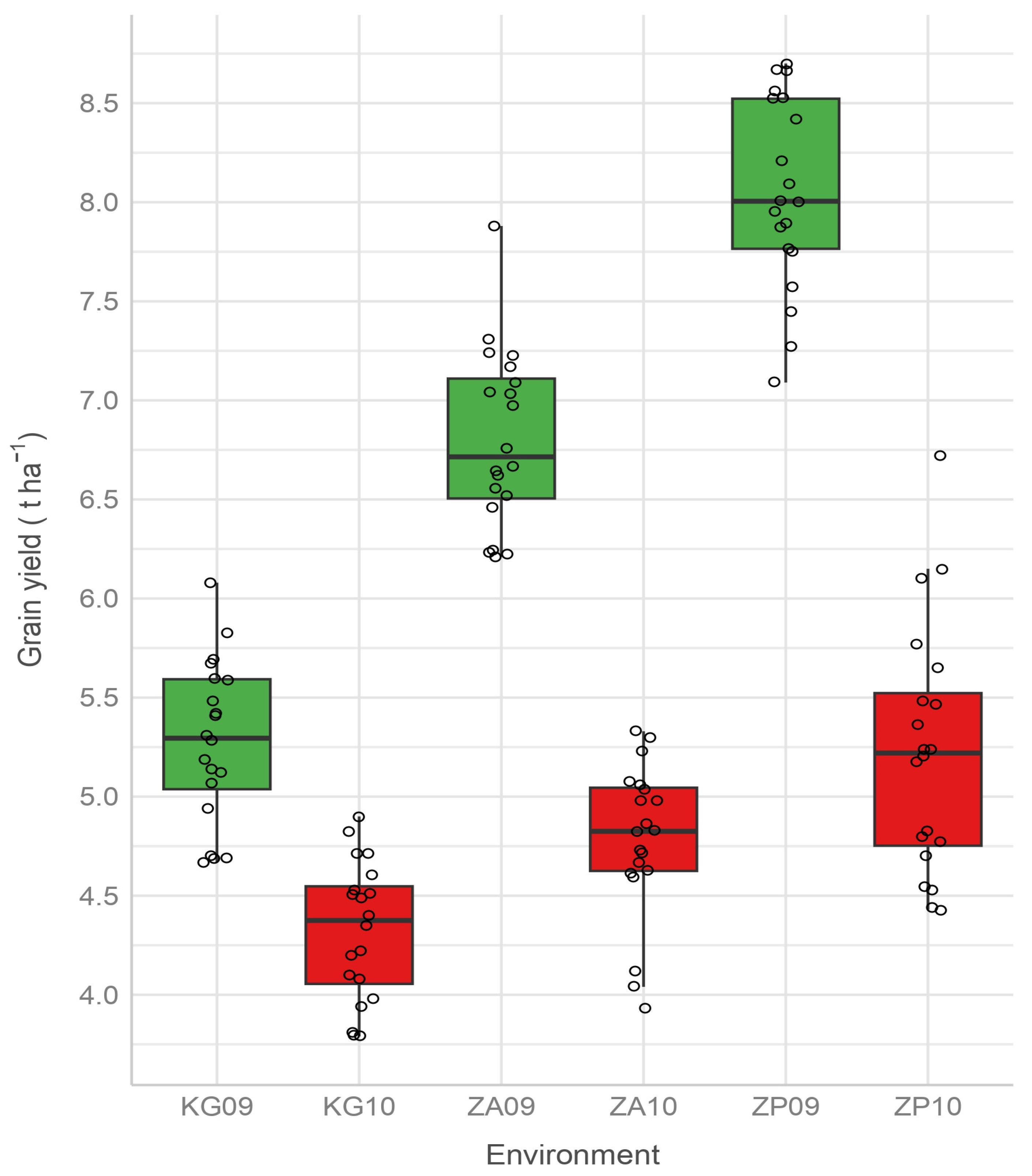
All the environments were low yielding and humid by the hydrothermal coefficient (htc > 2) in the second growing season. At the same time, they had lower values of the bioclimatic index. Reynolds et al. [19] also pointed out that precipitation may be a characteristic of low-yielding environments. However, in the first growing season, ZA09 was a high-yielding and humid environment (htc > 2), unlike ZP09 (high yielding) and KG09 (low yielding), which were optimally humid (1 ≤ htc ≥ 2). The values of these two indices for high-yielding environments ZP09 and ZA09 were between 1.82 (optimally humid) and 2.41 (humid) for htc and between 2.44 and 1.71 for bci, so the optimal values for the growth and development of barley are in this range. The possible explanation why KG09 (1.94 and 2.21, respectively) belongs to the group of low-yielding environments is that edaphic conditions at KG09 are probably poorer than in other investigated environments.

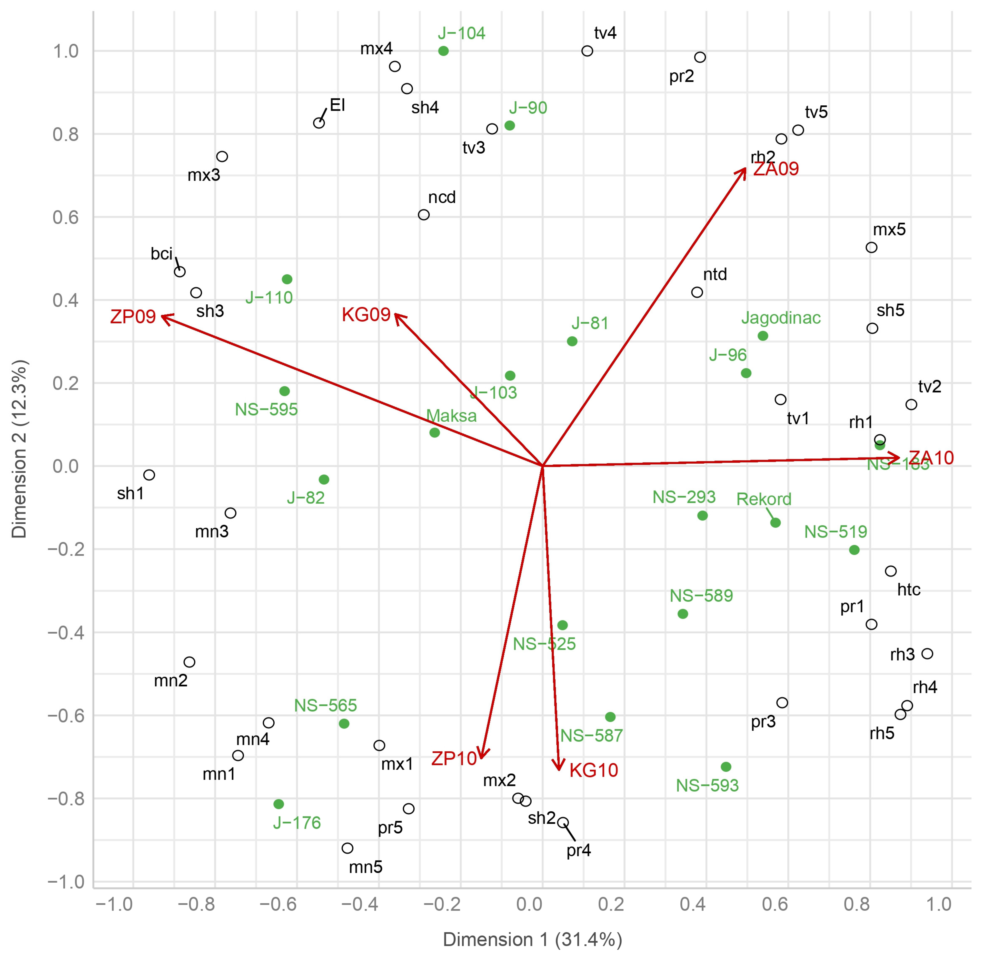
The results also showed that genotypes do not respond similarly to environmental variables at different stages of development, and therefore, we observed three clusters of genotypes. The first cluster consists of high-yielding genotypes NS-593, NS-565, and J-176 (two out of the three highest yielding) and one low-yielding genotype, NS-587. These genotypes represent younger genetic material created after 2000. They positively interacted with humid environments ZP10 and KG10 (recorded lodging of the stem). Based on the biplot display, it is suggested that these genotypes’ performances are associated with high precipitation during the spike growth stage onwards when barley is most sensitive to lodging, which can significantly reduce yields. This interaction can be partly explained by less sensitivity to lodging, which may be caused by lower stem height (all were low except J-176) or some other feature (wall thickness or more intense lignin production). Therefore, genotype J-176 may be a significant source of genes in further breeding due to its specific tolerance to lodging. These environments are also characterized by poor conditions for photosynthetic activity (negatively associated with temperatures and sun hours, as well as positively associated with relative humidity during April and May). However, the genotypes showed great stability regarding environmental effects on grain number and, especially, kernel weight determination in the spike growth and grain-filling stage. Csajbók et al. [72] indicate a large diversity in barley in terms of assimilation rate in poorer conditions for photosynthesis, which may be the reason for the better adaptability of these genotypes. These conditions reduced the positive temperature effect for grain number determination during the spike primordia stage in March.

The second cluster represented a group more sensitive to these conditions and consisted of high-yielding genotypes NS-595 and J-82 and low-yielding genotypes J-104, J-90, and J-110. All these genotypes belong to younger genetic material released after 2000. They had a positive interaction with optimally humid environments (ZP09 and KG09). This suggested that these genotypes favor highly moderate temperature conditions and sun hours in which assimilates are created (during the spike growth and grain-filling stage in April and May, respectively), which indicates that high yield was driven principally by kernel weight. These genotypes mostly had high and medium heights of the stem (except for J-90 and J-110). However, it was assumed that the interaction was partly a consequence of more sensitivity to the lodging of genotypes (except for J-110) in conditions represented in humid environments (ZP10 and KG10).

The third cluster consisted of three of the lowest-yielding genotypes, Jagodinac, Rekord, and NS-293, as well as high-yielding NS-183, NS-519, and J-96, which had a positive interaction with both humid environments in Zaječar. Except for the breeding line J-96, all cultivars were released before 2000 and represent older genetic material. Performances of these genotypes were associated with high temperatures and sun hours during June, as well as lower minimum temperatures during the whole season. Presumably, these genotypes were well adapted to warmer conditions during maturity. The earliness did not show any significance since positive interactions were realized with early (Jagodinac, NS-183, and Rekord), later (J-96 and NS-519), and medium-late (NS-293) genotypes. Dodig et al. [78] also confirms this claim by pointing out that two-row barley generally showed good adaptability to poorer weather conditions at the grain-filling and maturity stage, so that earliness is not as important as in six-row forms. These environments were characterized by low values of precipitation during these phases (pr4 and pr5), and therefore a lower probability of lodging, which explains the fact that the genotypes mostly had a taller stem (except NS-519 and Rekord). Therefore, better adaptability to these conditions of these genotypes we can explain by the high stem biomass. According to Savić et al. [79], a taller stem is related to high stem biomass, which determines the potential for accumulation and remobilization of dry matter from stem to grain in stress conditions. Less sensitivity to cold conditions (especially night) in stages during winter and spring is considered as important regarding genes for frost resistance. These genotypes showed stability under relatively poor environmental conditions concerning grain and spike number determination in the spike primordia stage during March (negatively correlated with mn2 and mx2, and positively with tv2).

Most genotypes showed a positive interaction with low-yielding and humid environments. These environments have affected both the highest-yielding (NS-525, J-176, and NS-593) and the lowest-yielding (Jagodinac, NS-293, and Rekord) genotypes. The same results were reached by Dodig et al. [78] and Hilmarsson et al. [80], who indicated better adaptability of two-row barley in low-yielding environments compared to six-row barley, which is more favorable in high-yielding environments.

The study of interaction is the basis for genotype selection intended for cultivation in wider geographical areas and for those intended for specific areas [81]. In our study, genotypes J-104, J-90, J-176, NS-565, and NS-593 had significant contributions to the interaction, which, according to Gauch [82], indicated that these genotypes were under more substantial influence of the environment. On the other hand, genotypes that showed a smaller contribution to the interaction reacted better to changes in external factors and are intended for growing in wider geographical areas, thus indicating stability. Elakhdar et al. [9] highlighted that in order to use the beneficial effects of the interaction and the selection of favorable barley genotypes to be more precise, the stability and average yield values should be considered. Thus, the identification of genotypes with wide adaptation would be possible. Therefore, genotypes NS-525, NS-589, and J-103 stand out for their stability and yield above the general average, so we can consider them widely adaptable and recommend them for all investigated localities.

In such cases, when the environments are location-year combinations, Zobel et al. [83] points out that a site suitable for prediction and recommendation is the one whose interaction effects slightly differ from year to year. Also, it is convenient for the environments to be more discriminating, i.e., informative, which corresponds to less stable environments. Except for KG09, all environments showed contributing interactions and discriminating effect, but KG09 and KG10, as well as ZP09 and ZP10, showed variations in interaction effect, which will cause changes in rank and absolute yield from year to year and will make the production recommendation more difficult. Zaječar, as a locality, is, therefore, the most suitable and the most reliable for examining grain yield, both due to the small difference in the interaction effect between its environments and due to the discriminating effect of both environments. The genotypes recommended for production in Zaječar are the following: Jagodinac, Rekord, NS-293, NS-183, NS-519, and J-96.

5. Conclusions

The largest number of variables showed their importance during May when the anthesis and filling stage took place in the climatic conditions of Serbia. During these phases, barley was generally the most sensitive to the environmental factors that cause interaction. During the spike primordia phase, only temperature variables showed importance. Temperature variables did not show significance only in the vegetative phase, but they had an indirect effect over the sun hours. Generally, the first season was moderately humid (based on precipitation) with a warm and sunny spring, while the second season was humid with a colder spring, which caused a significantly lower yield.

Information about differences among cultivars in sensitivity to environmental factors at different crop stages could be used to breed germplasm with less sensitivity to GEI if lines with complementary adaptation can be crossed and selected appropriately. Data related to the causes of interaction should be used to source genes for resistance to stress conditions. Weather data could be used in conjunction with long-term data to predict the relative yield stability of these crops in new environments or in response to climate change. Knowledge of statistically significant environmental and phenological factors in GEI enables the effectiveness of molecular research. Thus, our research indicates that the expression of crop developmental genes in the anthesis and grain-filling stage is important for understanding the interaction in two-row barley.

The variables used in this study are only part of a large number of factors that affect the expression of genotypes, which emphasizes the complexity of the interaction itself and the physiological processes that affect it. Also, the specific adaptations of the genotypes are partially explained by the characteristics of the genotypes, such as the height of the stem and resistance to lodging.

Using the PLSR model, superior genotypes can be singled out in terms of stability and average yield values (NS-525, NS-589, and J-103), as well as suitable localities for production recommendation and test location for selection and breeding purposes. In Kragujevac and Zemun Polje, the unpredictable crossover interactions dominated over the predictable ones. Such interactions are typically associated with years, which makes mega-environments less numerous and fewer advantages from specific adaptations could be taken. Zaječar is the most suitable and the most reliable of the studied localities for yield testing, and specific interactions were significant. Therefore, its environment can be considered as one mega-environment. Therefore, emphasize it as a specific location in relation to the other two and eastern Serbia in relation to other regions.

References

1. FAOSTAT Food and Agriculture Organization of the United Nations, FAOSTAT Statistical Database. Available online: https://www.fao.org/faostat/en (accessed on 29 December 2022).
2. SORS. Statistical Office of the Republic of Serbia. Available online: https://www.stat.gov.rs/ (accessed on 29 December 2022).
3. Kok, Y.; Ye, L.; Muller, J.; Ow, D.S.; Bi, X. Brewing with malted barley or raw barley: What makes the difference in the processes? Appl. Microbiol. Biotechnol. 2019, 103, 1059–1067. [Google Scholar] [CrossRef] [PubMed]
4. Newton, A.C.; Flavell, A.J.; George, T.S.; Leat, P.; Mullholland, B.; Ramsay, L.; Revoredo-Giha, C.; Russell, J.; Steffenson, B.J.; Swanston, J.S.; et al. Crops that feed the world 4. Barley: A resilient crop? Strengths and weaknesses in the context of food security. Food Secur. 2011, 3, 141–178. [Google Scholar] [CrossRef]
5. Monteverde, E.; Gutierrez, L.; Blanco, P.; De Vida, F.P.; Rosas, J.E.; Bonnecarrère, V.; Quero, G.; Mccouch, S. Integrating molecular markers and environmental covariates to interpret genotype by environment interaction in Rice (Oryza sativa L) grown in sub-tropical areas. Genome 2019, 9, 1519–1531. [Google Scholar] [CrossRef]
6. Herrera, J.M.; Levy, H.L.; Mascher, F.; Hiltbrunner, J.; Fossati, D.; Brabant, C.; Charles, R.; Pellet, D. Lessons from 20 years of studies of wheat genotypes in multiple environments and under contrasting production systems. Front. Plant Sci. 2020, 10, 1745. [Google Scholar] [CrossRef] [PubMed]
7. Senapati, A.K.; Goyari, P. Effect of Climate Variability on Yields of Major Crops Grown in Odisha, India. Ind. J. Agric. Econom. 2020, 75, 186–216. [Google Scholar]
8. Ullrich, S.E. Significance, adaptation, production and trade of barley. In Barley: Production, Improvement and Uses; Ullrich, S.E., Ed.; Blackwell Publishing Ltd.: Chichester, UK, 2011; pp. 3–13. [Google Scholar] [CrossRef]
9. Elakhdar, A.; Kumamaru, T.; Smith, K.; Robert, S.; Brueggeman, R.; Capo-Chichi, L.; Shyam Solanki, S. Genotype by Environment Interactions (GEI) for Barley Grain Yield Under Salt Stress Condition. J. Crop Sci. Biotechnol. 2017, 20, 193–204. [Google Scholar] [CrossRef]
10. de Leon, N.; Jannink, J.L.; Edwards, J.W.; Kaeppler, S.M. Introduction to a special issue on genotype by environment interaction. Crop Sci. 2016, 56, 2081–2089. [Google Scholar] [CrossRef]
11. Bocianowski, J.; Warzecha, T.; Nowosad, K.; Bathelt, R. Genotype by environment interaction using AMMI model and estimation of additive and epistasis gene effects for 1000-kernel weight in spring barley. J. Appl. Genet. 2019, 60, 127–135. [Google Scholar] [CrossRef]
12. Al-Tabbal, J. Genetic Variation, Heritability, Phenotypic and Genotypic Correlation Studies for Yield and Yield Components in Promising Barley Genotipes. J. Agric. Sci. 2012, 4, 193–210. [Google Scholar] [CrossRef]
13. Crossa, J.; Vargas, M.; van Eeuwijk, F.A.; Jiang, C.; Edmeades, G.; Hoisington, D. Interpreting genotype × environment interaction in tropical maize using linked molecular markers and environmental covariables. Theor. Appl. Genet. 1999, 99, 611–625. [Google Scholar] [CrossRef]
14. Zorić, M.; Terzić, S.; Sikora, V.; Brdar-Jokanović, M.; Vassilev, D. Effect of environmental variables on performance of Jerusalem artichoke (Helianthus tuberosus L.) cultivars in a long term trial: A statistical approach. Euphytica 2017, 213, 23. [Google Scholar] [CrossRef]
15. Alipour, H.; Abdi, H.; Rahimi, Y.; Bihamta, M.R. Genotype-by-year interaction for grain yield of Iranian wheat cultivars and its interpretation using Vrn and Ppd functional markers and environmental covariables. Cereal Res. Commun. 2021, 49, 681–690. [Google Scholar] [CrossRef]
16. Voltas, J.; Lopez-Corcoles, H.; Borras, G. Use of biplot analysis and factorial regression for the investigation of superior genotypes in multi-environment trials. Eur. J. Agron. 2005, 22, 309–324. [Google Scholar] [CrossRef]
17. Ozaktan, H.; Uzun, S.; Uzun, O.; Ciftci, C.Y. Assessment of Agro-Morphological Traits of Common Bean Genotypes Grown Under Organic Farming Conditions with Multi-Variate Analyses and Applications. Gesunde Pflanzen 2023, 75, 515–523. [Google Scholar] [CrossRef]
18. Elias, A.A.; Robbins, K.R.; Doerge, R.W.; Tuinstra, M.R. Half a century of studying genotype× environment interactions in plant breeding experiments. Crop Sci. 2016, 56, 2090–2105. [Google Scholar] [CrossRef]
19. Reynolds, M.P.; Trethowan, R.; Crossa, J.; Vargas, M.; Sayre, K.D. Physiological factors associated with genotype by environment interaction in wheat. Field Crops Res. 2002, 75, 139–160. [Google Scholar] [CrossRef]
20. Pacheco, A.; Vargas, M.; Alvarado, G.; Rodríguez, F.; Crossa, J.; Burgueño, J. GEA-R (Genotype × Environment Analysis with R for Windows) Version 4.0. CIMMYT Research Software, Mexico. 2015. Available online: https://hdl.handle.net/11529/10203 (accessed on 19 July 2021).
21. Vargas, M.; Crossa, J.; van Eeuwijk, F.A.; Ramirez, M.E.; Sayre, K. Using AMMI, factorial regression and partial least squares regression models for interpreting genotype x environment interaction. Crop Sci. 1999, 39, 955–967. [Google Scholar] [CrossRef]
22. Luedeling, E.; Gassner, A. Partial Least Squares Regression for analyzing walnut phenology in California. Agric. For. Meteorol. 2012, 158–159, 43–52. [Google Scholar] [CrossRef]
23. Porker, K.; Coventry, S.; Fettell, N.A.; Cozzolino, D.; Eglinton, J. Using a novel PLS approach for envirotyping of barley phenology and adaptation. Field Crops Res. 2020, 246, 107697. [Google Scholar] [CrossRef]
24. Borràs-Gelonch, G.; Salfer, G.A.; Casas, A.; van Eeuwijk, F.; Romagosa, I. Genetic control of pre-heading phases and other traits related to development in a double haploid barley population (Hordeum vulgare L.). Field Crops Res. 2010, 119, 36–47. [Google Scholar] [CrossRef]
25. Holzworth, D.P.; Huth, N.I.; Voil, P.G.; Zurcher, E.J.; Herrmann, N.I.; McLean, G.; Chenu, K.; van Oosterom, E.J.; Snow, V.; Murphy, C.; et al. APSIM—Evolution towards a new generation of agricultural systems simulation. Environ. Model. Softw. 2014, 62, 327–350. [Google Scholar] [CrossRef]
26. Dodig, D.; Rančić, D.; Vučelić Radović, B.; Zorić, M.; Savić, J.; Kandić, V.; Pećinar, I.; Stanojević, S.; Šešlija, A.; Vassilev, D.; et al. Response of wheat plants under postanthesis stress induced by defoliation: II. Contribution of peduncle morpho-anatomical traits and carbon reserves to grain yield. J. Agric. Sci. 2017, 155, 475–493. [Google Scholar] [CrossRef]
27. Kondić-Špika, A.; Mladenov, N.; Grahovac, N.; Zorić, M.; Mikić, S.; Trkulja, D.; Marjanović-Jeromela, A.; Miladinović, D.; Hristov, N. Biometric analyses of yield, oil and protein contents of wheat (Triticum aestivum L.) genotypes in different environments. Agronomy 2019, 9, 270. [Google Scholar] [CrossRef]
28. Chairi, F.; Aparicio, N.; Serret, M.D.; Araus, J.L. Breeding effects on the genotype× environment interaction for yield of durum wheat grown after the green revolution: The case of Spain. Crop J. 2020, 8, 623–634. [Google Scholar] [CrossRef]
29. Burstin, J.; Salloignon, P.; Chabert-Martinello, M.; Magnin-Robert, J.B.; Siol, M.; Jacquin, F.; Chauveau, A.; Pont, C.; Aubert, G.; Delaitre, C.; et al. Genetic diversity and trait genomic prediction in a pea diversity panel. BMC Genom. 2015, 16, 105. [Google Scholar] [CrossRef] [PubMed]
30. Zorić, M. Analysis of Genotype and Environment Interaction in Maize Breeding Using Multivariate Models. Ph.D. Thesis, University of Belgrade, Faculty of Agriculture, Belgrade, Serbia, 2008. [Google Scholar]
31. Balalić, I.; Zorić, M.; Branković, G.; Terzić, S.; Crnobarac, J. Interpretation of hybrid x sowing date interaction for oil content and oil yield in sunflower. Field Crops Res. 2012, 137, 70–77. [Google Scholar] [CrossRef]
32. Crusiol, L.G.T.; Nanni, M.R.; Furlanetto, R.H.; Sibaldelli, R.N.R.; Cezar, E.; Sun, L.; Foloni, J.S.S.; Mertz-Henning, L.M.; Nepomuceno, A.L.; Neumaier, N.; et al. Yield Prediction in Soybean Crop Grown under Different Levels of Water Availability Using Reflectance Spectroscopy and Partial Least Squares Regression. Rem. Sens. 2021, 13, 977. [Google Scholar] [CrossRef]
33. Republic Hydrometeorological Institute of Serbia. Available online: http://www.hidmet.gov.rs/ (accessed on 26 September 2010).
34. Petrović, N. Climatic parameters. In Meteorology and Climatology in Biotechnology. Prakticum; University of Belgrade, Faculty of Agriculture: Belgrade, Serbia, 2001; pp. 90–102. [Google Scholar]
35. Finlay, K.W.; Wilkinson, G.N. The Analysis of Adaptation in a Plant-Breeding Programme. Aust. J. Agric. Res. 1963, 14, 742–754. [Google Scholar] [CrossRef]
36. Oman, S.D. Multiplicative effects in mixed model analysis of variance. Biometrika 1991, 78, 729–739. [Google Scholar] [CrossRef]
37. Yan, W.; Rajcan, I. Prediction of cultivar performance based on single-versus multiple-year tests in soybean. Crop Sci. 2003, 43, 549–555. [Google Scholar] [CrossRef]
38. Aastveit, H.; Martens, H. ANOVA interactions interpreted by partial least squares regression. Biometrics 1986, 42, 829–844. [Google Scholar] [CrossRef]
39. Vargas, M.; Crossa, J.; Sayre, K.; Reynolds, M.; Ramirez, M.E.; Talbot, M. Interpreting treatment × environment interaction in wheat using partial least squares regression. Crop Sci. 1998, 38, 679–689. [Google Scholar] [CrossRef]
40. Stone, M. Cross—Validatory choice and assessment of statistical predictions (with Discussion). J. R. Stat. Soc. Ser. B 1974, 36, 111–148. [Google Scholar] [CrossRef]
41. Yan, W.; Hunt, L.A.; Sheng, Q.; Szlavnics, Z. Cultivar Evaluation and Mega-environment Investigation Based on the GGE Biplot. Crop Sci. 2000, 40, 597–605. [Google Scholar] [CrossRef]
42. Dodig, D.; Zorić, M.; Knežević, D.; Dimitrijević, B.; Šurlan-Momirović, G. Assessing wheat performance using enviromental information. Genetika 2007, 39, 413–425. [Google Scholar] [CrossRef]
43. R Core Team. R: A Language and Environment for Statistical Computing; Version 4.2.0 (2022-04-22 ucrt); R Foundation for Statistical Computing: Vienna, Austria, 2023; Available online: https://www.R-project.org/ (accessed on 6 December 2023).
44. Kelly, A.M.; Smith, A.B.; Eccleston, J.A.; Cullis, B.R. The accuracy of varietal selection using factor analytic models for multi-environment plant breeding trials. Crop Sci. 2007, 47, 1063–1070. [Google Scholar] [CrossRef]
45. Zhang, R.; Hu, X.A. Comparison of empirical BLUP with different considerations of residual error variance for genotype evaluation of multi-location trials. Span. J. Agric. Res. 2019, 17, e0701. [Google Scholar] [CrossRef]
46. Pržulj, N.; Momčilović, V. Cultivar × year interaction for winter malting barley quality traits. In Conventional and Molecular Breeding of Field and Vegetable Crops; Kobiljski, B., Ed.; Institute for Field and Vegetable Crops: Novi Sad, Serbia, 2008. [Google Scholar]
47. de San Celedonio, R.P.; Abeledo, L.G.; Miralles, D.J. Identifying the critical period for waterlogging on yield and its components in wheat and barley. Plant Soil 2014, 378, 265–277. [Google Scholar] [CrossRef]
48. Ploschuk, R.A.; Miralles, D.J.; Colmer, T.D.; Ploschuk, E.L.; Striker, G.G. Waterlogging of Winter Crops at Early and Late Stages: Impacts on Leaf Physiology, Growth and Yield. Front. Plant Sci. 2018, 9, 1863. [Google Scholar] [CrossRef]
49. Glamočlija, Đ. Production of barley. In Special Farming. Cereals and Grain Legumes; Draganić: Belgrade, Serbia, 2004; pp. 58–62. [Google Scholar]
50. McMaster, G.S. Phytomers, phyllochrons, phenology and temperate cereal development. J. Agric. Sci. 2005, 143, 137–150. [Google Scholar] [CrossRef]
51. Mirosavljević, M.; Momčilović, V.; Maksimović, I.; Putnik-Delić, M.; Pržulj, N.; Hristov, N.; Mladenov, N. Preanthesis development of winter wheat and barley and relationships with grain yield. Plant Soil Environ. 2018, 64, 310–316. [Google Scholar] [CrossRef]
52. Abbate, P.E.; Andrade, F.H.; Culot, J.P.; Bindraban, P.S. Grain yield in wheat: Effects of radiation during spike growth period. Field Crops Res. 1997, 54, 245–257. [Google Scholar] [CrossRef]
53. Calderini, D.F.; Savin, R.; Labeled, O.G.; Reynolds, M.P.; Slafer, G.A. The importance of the period immediately preceding anthesis for grain weight determination in wheat. Euphytica 2001, 119, 199–204. [Google Scholar] [CrossRef]
54. Pržulj, N.; Mirosavljević, M.; Čanak, P.; Zorić, M.; Boćanski, J. Evaluation of spring barley performance by biplot analysis. Cereal Res. Commun. 2015, 43, 692–703. [Google Scholar] [CrossRef]
55. Voltas, J.; van Eeuwijk, F.A.; Araus, J.L.; Romagosa, I. Integrating statistical and ecophysiological analysis of genotype by environment interaction for grain filling of barley in Mediterranean areas II. Grain growth. Field Crops Res. 1999, 62, 75–84. [Google Scholar] [CrossRef]
56. Arisnabarreta, S.; Miralles, D.J. Critical period for grain number establishment of near isogenic lines of two- and six-rowed barley. Field Crops Res. 2008, 107, 196–202. [Google Scholar] [CrossRef]
57. Pradhan, G.P.; Prasad, P.V.V.; Fritz, A.K.; Kirkham, M.B.; Gill, B.S. Effects of drought and high temperature stress on synthetic hexaploid wheat. Funct. Plant Biol. 2012, 39, 190–198. [Google Scholar] [CrossRef] [PubMed]
58. Pržulj, N.; Grujić, O.; Momčilović, V.; Đurić, V.; Pejin, J. Malting barley in conditions of high air temperatures and drought. Zbornik Radova Instituta Ratarstvo Povrtarstvo 2005, 41, 313–321. [Google Scholar]
59. Pržulj, N.; Momčilović, V. Spring barley performances in the Pannonian zone. Genetika 2012, 44, 499–512. [Google Scholar] [CrossRef]
60. Arenas-Corraliza, M.G.; Rolo, V.; López-Díaz, M.L.; Moreno, G. Wheat and barley can increase grain yield in shade through acclimation of physiological and morphological traits in Mediterranean conditions. Sci. Rep. 2019, 9, 9547. [Google Scholar] [CrossRef]
61. Liu, W.G.; Sajad, H.; Liu, T.; Zou, J.L.; Ren, M.L. Shade stress decreases stem strength of soybean through restraining lignin biosynthesis. J. Integr. Agric. 2019, 8, 43–53. [Google Scholar] [CrossRef]
62. Li, C.H.; Luo, Y.L.; Jin, M.; Sun, S.F.; Wang, Z.L.; Li, Y. Response of Lignin Metabolism to Light Quality in Wheat Population. Front. Plant Sci. 2021, 12, 729647. [Google Scholar] [CrossRef] [PubMed]
63. Yu, M.Z.; Wang, M.; Gyalpo, T.; Basang, Y. Stem lodging resistance in hulless barley: Transcriptome and metabolome analysis of lignin biosynthesis pathways in contrasting genotypes. Genomics 2020, 113, 935–943. [Google Scholar] [CrossRef] [PubMed]
64. Sallam, A.; Alqudah, A.M.; Dawood, M.F.A.; Baenziger, P.S.; Börner, A. Drought stress tolerance in wheat and barley: Advances in physiology, breeding and genetics research. Int. J. Mol. Sci. 2019, 20, 3137. [Google Scholar] [CrossRef]
65. Stratonovitch, P.; Semenov, M.A. Heat tolerance around flowering in wheat identified as a key trait for increased yield potential in Europe under climate change. J. Exp. Bot. 2015, 66, 3599–3609. [Google Scholar] [CrossRef]
66. Ahakpaz, F.; Abdi, H.; Neyestani, E.; Hesami, A.; Mohammadi, B.; Mahmoudi, K.N.; Abedi-Asl, G.; Noshabadi, M.R.J.; Ahakpaz, F.; Alipour, H. Genotype-by-environment interaction analysis for grain yield of barley genotypes under dryland conditions and the role of monthly rainfall. Agric. Water Manag. 2021, 245, 106665. [Google Scholar] [CrossRef]
67. Pržulj, N.; Momčilović, V. Importance of spikelet formation phase in the yield biology of winter barley. Field Veg. Crop. Res. 2011, 48, 37–48. [Google Scholar] [CrossRef]
68. Kandić, V.; Dodig, D.; Sečanski, M.; Prodanović, S.; Branković, G.; Titan, P. Grain yield, agronomic traits, and protein content of two- and six-row barley genotypes under terminal drought conditions. Chil. J. Argric. Res. 2019, 79, 648–657. [Google Scholar] [CrossRef]
69. Caierão, E. Effect of induced lodging on grain yield and quality of brewing barley. Crop Breed. Appl. Biotechnol. 2006, 6, 215–221. [Google Scholar] [CrossRef]
70. Berry, P.M.; Spink, J. Predicting yield losses caused by lodging in wheat. Field Crops Res. 2012, 137, 19–26. [Google Scholar] [CrossRef]
71. Bai, Y.; Zhang, J.; Wu, Y.; Huang, R.; Chang, Y.; Lei, X.; Song, X.; Pei, D. Possibility of Increasing the Growth and Photosynthetic Properties of Precocious Walnut by Grafting. Sustainability 2020, 12, 5178. [Google Scholar] [CrossRef]
72. Csajbók, J.; Pepó, P.; Kutasy, E. Photosynthetic and Agronomic Traits of Winter Barley (Hordeum vulgare L.) Varieties. Agronomy 2020, 10, 1999. [Google Scholar] [CrossRef]
73. Slafer, G.A. Genetic basis of yield as viewed from a crop physiologist’s perspective. Ann. Appl. Biol. 2003, 142, 117–128. [Google Scholar] [CrossRef]
74. Majoul-Haddad, T.; Bancel, E.; Martre, P.; Triboi, E.; Branlard, G. Effect of short heat shocks applied during grain development on wheat (Triticum aestivum L.) grain proteome. J. Cereal Sci. 2013, 57, 486–495. [Google Scholar] [CrossRef]
75. Jacott, C.N.; Boden, S.A. Feeling the heat: Developmental and molecular responses of wheat and barley to high ambient temperatures. J. Exp. Bot. 2020, 71, 5740–5751. [Google Scholar] [CrossRef] [PubMed]
76. García, G.A.; Serrago, R.A.; Dreccer, M.F.; Miralles, D.J. Post-anthesis warm nights reduce grain weight in field-grown wheat and barley. Field Crops Res. 2016, 195, 50–59. [Google Scholar] [CrossRef]
77. Sadok, W.; Jagadish, S.V.K. The Hidden Costs of Nighttime Warming on Yields. Trends Plant Sci. 2020, 25, 644–651. [Google Scholar] [CrossRef]
78. Dodig, D.; Kandić, V.; Zorić, M.; Nikolić-Ðorić, E.; Tančić Živanov, S.; Perović, D. Response of kernel growth of barley genotypes with different row type to climatic factors before and after inflection point of grain filling. Field Crops Res. 2020, 255, 107864. [Google Scholar] [CrossRef]
79. Savić, J.; Kandić, V.; Rančić, D.; Pećinar, I.; Šešlija, A.; Ivanović, D.; Bratković, K.; Dodig, D. Association of agronomical, morphological and anatomical traits with compensatory effect of stem reserve mobilization in common wheat genotypes under drought stress. Ital. J. Agrometeorol. 2017, 22, 5–12. [Google Scholar] [CrossRef]
80. Hilmarsson, H.S.; Rio, S.; Sánchez, J.I. Genotype by Environment Interaction Analysis of Agronomic Spring Barley Traits in Iceland Using AMMI, Factorial Regression Model and Linear Mixed Model. Agronomy 2021, 11, 499. [Google Scholar] [CrossRef]
81. Petrović, S.; Dimitrijević, M.; Belić, M.; Banjac, B.; Bošković, J.; Zečević, V.; Pejić, B. The variation of yield componenets in wheat (Triticum aestivum L.) in response to stressful growing conditions of alkaline soil. Genetika 2010, 42, 545–555. [Google Scholar] [CrossRef]
82. Gauch, H.G. Statistical analysis of yield trials by AMMI and GGE. Crop Sci. 2006, 46, 1488–1500. [Google Scholar] [CrossRef]
83. Zobel, R.W.; Wright, M.J.; Gauch, H.G. Statistical analysis of a yield trial. Agron. J. 1988, 80, 388–393. [Google Scholar] [CrossRef]
Figure 1. Box plots for grain yield of two-row barley genotypes. Note: KG09, ZP09, and ZA09—Kragujevac, Zemun Polje, and Zaječar in 2008/2009, respectively; KG10, ZP10, and ZA10—Kragujevac, Zemun Polje, and Zaječar in 2009/2010, respectively.
Agronomy 14 00194 g001
Figure 2. PLSR biplot for grain yield of two-row barley genotypes. Note: mn1, mx1, tv1, pr1, rh1, sh1—average minimum and maximum temperature, average temperature variation, sum of precipitation, average relative humidity, number of sun hours in period November–February; mn2, mx2, tv2, pr2, rh2, sh2—same parameters in March; mn3, mx3, tv3, pr3, rh3, sh3—same parameters in April; mn4, mx4, tv4, pr4, rh4, sh4—same parameters in May; mn5, mx5, tv5, pr5, rh5, sh5—same parameters in June, respectively; EI—environmental index, bci—bioclimatic index, htc—hydrothermal coefficient, ntd—number of tropical days, ncd—number of cold days; KG09, ZP09, and ZA09—Kragujevac, Zemun Polje, and Zaječar in 2008/2009, respectively, KG10, ZP10, and ZA10—Kragujevac, Zemun Polje, and Zaječar in 2009/2010, respectively.
Agronomy 14 00194 g002
Figure 3. Spearman’s coefficient correlation among environmental variables. Note: mn1, mx1, tv1, pr1, rh1, sh1—average minimum and maximum temperature, average temperature variation, sum of precipitation, average relative humidity, number of sun hours in period November–February; mn2, mx2, tv2, pr2, rh2, sh2—same parameters in March; mn3, mx3, tv3, pr3, rh3, sh3—same parameters in April; mn4, mx4, tv4, pr4, rh4, sh4—same parameters in May; mn5, mx5, tv5, pr5, rh5, sh5—same parameters in June, respectively; EI—environmental index, bci—bioclimatic index, htc—hydrothermal coefficient, ntd—number of tropical days, ncd—number of cold days. Circle sizes represent the significance of correlations between the variables, with larger circles in darker shades indicating stronger positive or negative associations, and smaller circles in lighter shades suggesting weaker associations.
Agronomy 14 00194 g003