
Stacking Ensemble-Based Machine Learning Model for Predicting Deterioration Components of Steel W-Section Beams


1
Department of Civil Engineering, Zanjan Branch, Islamic Azad University, Zanjan 45156-58145, Iran
2
Department of Computer Engineering, Zanjan Branch, Islamic Azad University, Zanjan 45156-58145, Iran
*
Author to whom correspondence should be addressed.
Buildings 2024, 14(1), 240; https://doi.org/10.3390/buildings14010240 (registering DOI)
Original submission received: 17 November 2023
/
Resubmission received: 19 December 2023
/
Revised: 9 January 2024
/
Accepted: 12 January 2024
/
Published: 16 January 2024
(This article belongs to the Special Issue Mechanical Performance of Steel and Composite Beams)
Abstract
:The collapse evaluation of the structural systems under seismic loading necessitates identifying and quantifying deterioration components (DCs). In the case of steel w-section beams (SWSB), three distinct types of DCs have been derived. These deterioration components for steel beams comprise the following: pre-capping plastic rotation (θp), post-capping plastic rotation (θpc), and cumulative rotation capacity (Λ). The primary objective of this research is to employ a machine learning (ML) model for accurate determination of these deterioration components. The stacking model is a powerful combination of meta-learners, which is used for better learning and performance of base learners. The base learners consist of AdaBoost, Random Forest (RF), and XGBoost. Among various machine learning algorithms, the stacking model exhibited superior functioning. The evaluation metrics of the stacking model were as follows: R2 = 0.9 and RMSE = 0.003 for θp, R2 = 0.97 and RMSE = 0.012 for θpc, and R2 = 0.98 and RMSE = 0.09 for Λ. The significance of input variables, specifically the web-depth-over-web-thickness ratio (h/tw) and the flange width-to-thickness ratio (bf/2tf), in determining the deterioration components was assessed using the Shapley Additive Explanations model. These parameters emerged as the most crucial factors in the evaluation.
Keywords:
deterioration components; machine learning; AdaBoost; random forest; XGBoost; stacking; steel beams1. Introduction
Nowadays, there has been a growing trend in employing machine learning techniques to address challenges in the domain of seismic and structural engineering. Machine learning offers the potential to supplant the reliance on current empirical and semi-empirical prediction models, offering the advantage of highly accurate models. A novel artificial intelligence approach, known as ICA–XGBoost, has been employed in studies to forecast the strength of concrete containing recycled aggregates. This method combines the utilization of a meta-heuristic algorithm called ICA with the machine learning algorithm XGBoost. The outcomes demonstrated that this amalgamated algorithm outperformed other algorithms, yielding superior results [1]. A comprehensive investigation was conducted to explore the expanding applications of machine learning in the subject of structural engineering. The research encompassed a systematic review of various machine learning techniques, machine learning libraries, as well as Python resources, codes, and datasets pertinent to structural engineering [2]. A scholarly discussion centered on implementing a machine learning approach to calculate and optimize the modulus of elasticity of concrete containing recycled aggregates. A comparative analysis was conducted to assess the performance of the ensemble model against other algorithms, revealing that the ensemble model exhibited more precise predictions than the individual models [3]. The algorithms of machine learning were utilized to predict the shear strength of beams containing concrete with recycled aggregates, both with and without shear reinforcement. The shear strength of reinforced concrete elements is obtained using the XGBoost model [4,5,6]. In addition, researchers utilized an ensemble learning method to forecast the shear strength of deep reinforced concrete beams, both with and without reinforced web. The findings revealed that the ensemble method outperformed traditional machine learning methods, presenting a superior performance [7].
Consumption of recycled aggregates as a replacement for natural aggregates in concrete preparation is recognized as an operative means to promote sustainability within the construction industry. Liu et al. [8] applied machine learning models to forecast the stability of concrete containing recycled aggregates. The outcomes revealed that the artificial neural network (ANN) model achieved the uppermost level of predictive accuracy. Hu and Kwok [9] employed machine learning techniques to predict the wind pressure distribution around circular cylinders. They found that the gradient boosting regression trees model had the most pronounced impact on predictive performance.
Pyakurel et al. [10] employed machine learning techniques to predict landslides activated by seismic actions. The conclusions revealed that the trees classifier model exhibited a greater efficacy compared to other models. Feng et al. [11] investigated the uncertainty of machine learning models when assessing the sensitivity of landslides caused by earthquakes. In assessing the design strength of cement-stabilized soft soil (cement soil) across diverse application environments, several field and indoor geotechnical tests are typically managed. However, these experiments often lead to inefficiencies in terms of resource utilization, cost, and time, while also posing significant environmental pollution challenges. The compressive strength of cement, the strength and hardness of cement-stabilized soils, has been obtained using different machine learning methods. The obtained results display that machine learning models are highly accurate in predicting the compressive strength of cement [12,13,14].
Sayed et al. [15] conducted a study utilizing machine learning models to forecast the axial compressive load of concrete columns with FRP encasement. They reported that the gradient boosting and random forest models achieved the highest accuracy in prediction. Nguyen and Ly [16] conducted compressive strength and sensitivity analyses of fiber-reinforced self-compacting concrete (FRSCC) using machine learning models. The outcomes indicated that XGBoost exhibited the highest predictive performance. The estimation of mechanical properties of concrete is often a crucial requirement in design codes. The introduction of novel concrete mixes and applications has prompted scientists to seek reliable models for predicting mechanical strength. Chaabene et al. [17] employed machine learning methods to predict the mechanical properties of concrete. Jiang and Zhao [18] applied machine learning methods to the design of stainless steel bolted connections. The obtained results showed that the support vector machine has the finest accuracy and performance.
In the other study, the chloride diffusion coefficient of concrete is predicted by Taffese and Espinosal-Leal [19] based on machine learning techniques. The outcomes revealed that the XGBoost model demonstrated the most predictive performance. Mousavi et al. [20] applied machine learning methods to categorize the properties of wood derived from ultrasonic tests. Li et al. [21] successfully determined the compressive strength of BFRC by a combined algorithm of kernel extreme learning machine (KELM) and genetic algorithm (GA). They found that the KELM–GA model exhibited strong predictive capabilities.
Sandeep et al. [22] utilized machine learning techniques to predict the shear strength of reinforced concrete beams, presenting the capabilities of this approach. Kaveh et al. [23] employed machine learning methods to predict the shear strength of FRP-reinforced concrete girders. They observed that the extreme gradient boosting model outperformed other machine learning models, demonstrating its superior predictive capabilities. Artificial neural networks (ANN) are used to determine the shear strength of flexural members reinforced, cold-formed steel structures and complex deformation of structural elements [24,25,26].
Jiang et al. [27] obtained the deterioration of a bridge through the hybrid method of whale algorithm with other machine learning. The results demonstrated that the combined model performed better than the simple model. Hwang et al. [28] utilized machine learning models to predict seismic responses and classify structural collapse for ductile reinforced concrete buildings during seismic events, effectively accounting for the inherent uncertainty. The compressive strength can differ depending on the composition and ratio of the components and materials employed. Farooq et al. [29] employed machine learning methods for high-performance prediction. The results indicated that the function of bagging and boosting methods had enhanced the response of the basic machine learning models. Concrete-encased steel columns (CES), commonly referred to as concrete and steel composite columns, exhibit excellent fire resistance attributed to the performance of concrete. Li et al. [30] utilized the artificial neural network method to forecast fire resistance in composite columns. Predicting the nominal shear capacity of deep reinforced concrete beams with openings poses a complex challenge due to its highly nonlinear behavior. Li et al. [31] investigated the progressive collapse performance of the planar frame structure with engineered cementation composites (ECC) under the removal of the middle column for normal concrete and ECC samples. The results have shown that the (ECC) sample has limited cracking, and progressive collapse performance is also improved. Li and Song [32] utilized the stacking ensemble learning method to forecast the compressive strength of concrete incorporating rice husk ash. The results demonstrated that the proposed new model exhibited a superior performance compared to other algorithms.
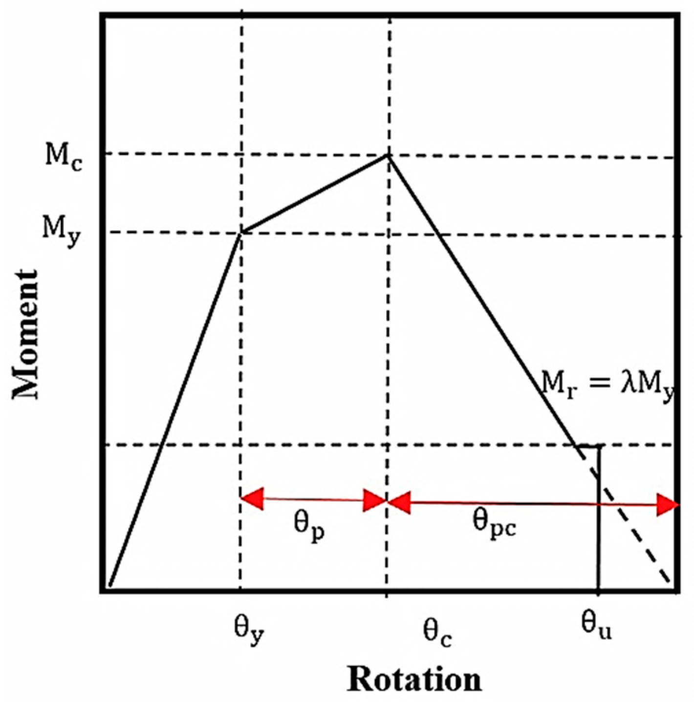
This paper will use machine learning techniques for the prediction of deterioration components (DCs) of steel w-section beams. The source data are related to a Lignos and Krawinkler [33] study that utilized analytical relations based on experimental tests to ascertain the deterioration components of steel w-section beams data, namely Pre-capping plastic rotation (θp, post-capping plastic rotation(θpc), and cumulative rotation capacity (Λ). These parameters are critical for the collapse evaluation of structural elements that require effective hysteretic models capable of summarizing the failure behavior of structural components. Backbone curves delineate the boundaries of the hysteretic response of these components, as depicted schematically in Figure 1.
In this study, DCs are predicted through a stacking model. Specifically, three base learners, namely AdaBoost, Random Forest (RF), and XGBoost, are selected as primary predictors, with RF used as the meta-learner in the stacking model. Hyperparameter optimization is conducted using grid search and 5-fold cross-validation methods. The importance of features is assessed through the Shapley Additive Explanations model. The dataset comprises 157 laboratory samples pertaining to steel w-section beams, which were collected by Lignos and Krawinkler [33]. Empirical relationships presented by Lignos and Krawinkler are considered for predicting DCs. A comparison between these empirical relationships and machine learning models reveals that the stacking model exhibits remarkable accuracy and performance.
2. Overview of the Machine Learning Techniques
2.1. Random Forest
Random forest is a user-friendly machine learning algorithm known for delivering highly satisfactory results even without fine-tuning its meta-parameters. Owing to its straightforwardness and practicality, this algorithm is widely regarded as one of the most frequently employed machine learning methods for both classification and regression tasks. Random forest is a supervised learning algorithm that derives its name from the creation of a random forest. The forest itself is essentially a collection of decision trees generated using the “bagging” method. This approach involves combining multiple learning models to boost the overall performance of the model. In essence, the random forest constructs numerous decision trees and integrates them to yield more precise and stable predictions. A key advantage of the random forest algorithm lies in its versatility, as it can be effectively employed for both classification and regression tasks, which form the core of numerous contemporary machine learning systems. The impressive performance of random forest has been extensively validated through comprehensive research studies.
The random forest model can be shown as below:
In the context of a random forest, represents a single-tree learner that relies on a randomly selected subset of training data of size d, chosen using (f) features. Each tree, denoted as (k), yields a corresponding leaf. Hence, the three key parameters for the random forest are f, k, and d [34].
2.2. AdaBoost
AdaBoost, standing for Adaptive Boosting, represents a pioneering boosting algorithm primarily designed for binary classification tasks. It serves as an excellent entry point for grasping the fundamentals of boosting concepts. Additionally, contemporary boosting techniques, such as stochastic gradient boosting machines, are built on the principles of AdaBoost. The overall boosting method is based on AdaBoost, including random boosting machines. The form of its receiver is as follows:
In each iteration, a novel learner is employed to assess all samples that constitute the training set. The misclassified sample’s weight is augmented, while the correctly classified sample’s weight diminishes. With each iteration, a new weak learner is generated, and it is allocated a coefficient to minimize the training error of the ensemble.
In this context, denotes the learner constructed from previous training iterations. E(0) represents an error function, and corresponds to a weak learner, aiding the strong learner. In the adaptive reinforcement approach, the amalgamation of multiple weak learners contributes to the formation of a robust and powerful learner [35].
2.3. XGBoost
The XGBoost algorithm is a recently employed process in the domain of machine learning. It serves as an implementation of decision tree gradient boosting specifically developed for achieving high speed and efficiency. Utilizing the XGBoost algorithm enables us to enhance computational efficiency in terms of calculation time and memory utilization. Further, this algorithm is designed to optimize the utilization of available resources during model training. The objective function in XGBoost can be represented as follows:
In this context, L denotes the cost function of the bias model, while ω signifies the regularization term aimed at mitigating model complexity. The XGBoost algorithm employs gradient-boosted decision trees, which effectively enhance both speed and performance. Further, the inclusion of the regularization term in this method aids in preventing overfitting [36].
2.4. Stacking
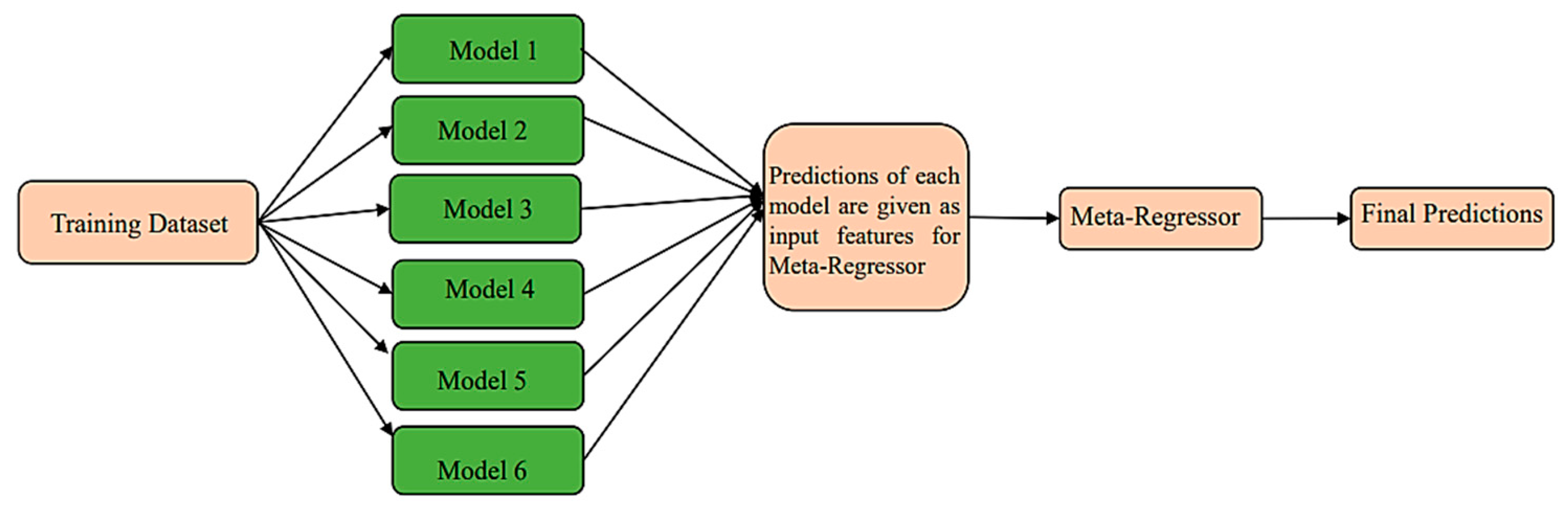
Hybrid machine learning models are one of the machine learning models. In these methods, weak learner models or base learner models are trained to solve a problem and combined to achieve better results. When weak models are appropriately combined with each other, they can generate more precise or stable models. The selection of appropriate algorithms is a critical factor in achieving favorable outcomes within machine learning models. The choice of model rests on many variables in the problem, such as the extent of data, the dimensions of the data, and the distribution hypothesis. Having a model with low bias and variance are two essential and required features. In hybrid machine learning methods, base learners are combined with each other to create more complex models. Frequently, these individual models do not exhibit satisfactory performance in isolation, owing to their inherently high bias or variance. The stacking method is one of the techniques employed to integrate elementary models effectively [37]. The stacking model uses a heterogeneous model and different machine learning algorithms. Additionally, the stacking method combines base models with each other using meta-models and provides better prediction. When the base models (traditional empirical models) are properly combined with each other, the result can create more precise or stable models. The core principle behind stacking involves training multiple diverse basic models and subsequently employing a meta-model to combine their predictions, thus yielding the final prediction. To establish a stacking model, two essential components are required: (1) basic models, trained on the training data, and (2) a meta-model designed to amalgamate the outcomes of the basic models. In the stacking learning algorithm, the meta-learner training set is derived from the base learner training. Use of the results obtained from the base learner may lead to overfitting when applied to the new training set of the meta-learner. To address this issue, k-fold cross-validation is employed. The stacking model is shown schematically in Figure 2.
2.5. k-Fold Cross-Validation
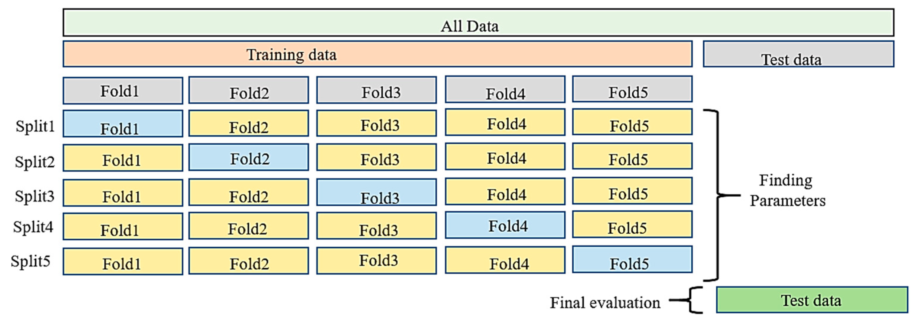
In scenarios where the training data in a machine learning problem are relatively limited, or the results pertaining to the test data are not highly precise, it becomes essential to conduct multiple tests and subsequently average the outcomes for the final evaluation. In such cases, the cross-validation method is employed, wherein the data are divided into K subsets. Subsequently, in K different iterations, one of the K subsets is designated as the test set, while the remaining K-1 subsets function as the training data. Ultimately, the evaluation results are averaged to yield the final evaluation outcome. Cross-validation serves as a standard technique to assess the performance of a machine learning algorithm on a dataset. An important aspect of this method involves exploring the impact of different values for the parameter “k” when estimating model performance and comparing it with the outcomes under ideal test conditions. This helps in determining the appropriate value for “k”. The k-fold method incorporates a parameter denoted as “k,” representing the number of groups into which a given data sample is to be partitioned. Once a specific value for “k” is chosen, it may be referenced accordingly, such as k = 5, indicating 5-fold cross-validation [38]. The following Figure 3 shows the mentioned cross-validation schematically.
2.6. Grid Search
Model parameters are characteristics of the training data that are acquired and fine-tuned during the training process using machine learning algorithms. Examples of model parameters include the slope and width from the origin in linear regression. Note that model parameters vary across different experiments and are contingent upon the specific dataset as well as the nature of the problem being referred. On the other hand, hyperparameters must be predetermined and specified by the data scientist before the training phase commences. The Scikit-Learn Python library (or its counterparts in other software) provides default hyperparameters for each model. However, these default values may not be optimal for our specific problem. Finding the best hyperparameters is often challenging, but through experience and iterative testing, one can eventually identify the most suitable values. This necessitates conducting experiments and evaluating the performance of each model resulting from a large number of hyperparameter combinations. To obtain the optimal hyperparameters, one commonly employed approach is the grid search method. Unlike random search, grid search systematically evaluates all possible combinations of hyperparameter values within specified ranges, thereby making the search space more comprehensive and exhaustive [39].
3. Research Significance
The primary objective of earthquake engineering has always been to comprehend, predict, and prevent structural collapse. From a financial perspective, collapse refers to a state in which a building, its contents, and its functionality are utterly destroyed, leading to significant monetary loss. Moreover, collapse poses a threat to human safety, resulting in injuries and fatalities. Thus, it becomes imperative to evaluate the level of life safety, as it is a fundamental general concern. The assessment of structural collapse necessitates the use of hysteretic models capable of capturing the failures occurring in structural components. Backbone curves, representing the boundaries of hysteretic response, serve as a means to depict the deterioration components within structural members, as depicted schematically in Figure 1. The deterioration components, encompassing θp = pre-capping plastic rotation, θpc = post-capping plastic, and Λ = cumulative rotation capacity, have a key role in providing necessary information about the deterioration characteristics of steel moment-resisting frames. To obtain comprehensive data regarding these parameters, a collection of laboratory tests is imperative. The dataset comprises 157 tests of steel w-section beams, thoughtfully compiled by Lignos and Krawinkler [33]. Using experimental data, empirical relationships have been obtained for two types of beams: beams with other than reduced beam section (RBS) and beams with RBS [33]. The resulting relationships are as follows:
Beams other than RBS:
θp=0.318(h/tw)−0.55∙(bf/2tf)−0.345∙(Lb/ry)−0.023∙(L/d)0.09∙(c1unit∙d/533)−0.33 (c2unit∙Fy/355)−0.13
θpc=7.5(h/tw)−0.61(bf/2tf)−0.71 (Lb/ry)−0.11 (c1unit.d/533)−0.161 (c2unit∙Fy/355)−0.32
Λ=536(h/tw)−1.26 (bf/2tf)−0.525 (Lb/ry)−0.13 (c2unit∙Fy/355)−0.291
Beams with RBS:
θp=0.19(h/tw)−0.314 (bf/2tf)−0.1 (Lb/ry)−0.185 (L/d)0.113 (c1unit∙d/533)−0.76 (c2unit∙Fy/355)−0.07
θpc=9.52(h/tw)−0.513 (bf/2tf) −0.863 (Lb/ry)−0.108 (c2unit∙Fy/355)−0.36
Λ=585∙(h/tw)−1.14 (bf/2tf)−0.632 (Lb/ry)−0.205 (c2unit∙Fy/355)−0.391
The analytical relationships are derived from considerations of geometrical characteristics and material properties. These relations specifically pertain to sections of the W-section type. The resulting analytical equations encompass the following parameters:
h/tw is the web-depth-over-web-thickness ratio, Lb/ry is the ratio between beam unbraced length Lb over a radius of gyration, bf/2tf is the flange width-to-thickness ratio used for compactness, L/d is the shear span-to-depth ratio of the beam, d is the beam depth of the cross section, Fy is the expected yield strength of the flange of the beam, which is normalized by 50 ksi (typical nominal yield strength of structural us steel), and C1unit and C2unit are coefficients for unit conversion. They both are 1 if inches and ksi are used, and they are C1unit = 0.0254 and C2unit = 0.145 if d is the meter and Fy is in MPa.
This research employs machine learning techniques to determine the deterioration components of w-section steel beams. As Lignos and Krawinkler [33] used five numbers of parameters (h/tw, bf/2tf, L/d, d, Lb/ry), these parameters have the most effect on the deterioration components. But the number of experimental data had similar input parameters; therefore, machine learning models made mistakes in training. For this purpose, three parameters (connection type, test configuration, and yield moment) have been added to the input. In addition to the parameters proposed by Lignos and Krawinkler [33], this study introduces three additional parameters, namely connection type, test configuration, and yield moment (MY). The connection type encompasses approximately 29 distinct connection types, as detailed in Table 1, while the test configuration includes around 8 different configurations listed in Table 2. To incorporate the connection type and test configuration into the machine learning models, each type is assigned a corresponding label. For instance, the 29 connection types are designated with numbers 1 to 29, and the 8 formation types are assigned numbers 1 to 8 [40].
4. Data Preprocessing
The current investigation centers around a dataset derived from laboratory experiments [33]. The number of laboratory data is 157. Among the 157 data, some data are similar, and some others are not reported, so the averaging method has been used for the data. Thus, there are 96 samples available for θp, 91 samples for θpc, and 96 samples for Λ. The experimental collected data can be accessed in the Lignos thesis dissertation [40]. The input data considered in this study encompass several factors, including the web-depth-over-web-thickness ratio (h/tw), the ratio between beam unbraced length Lb over a radius of gyration (Lb/ry), the flange width-to-thickness ratio used for compactness (bf/2tf), the shear span-to-depth ratio of the beam (L/d), the beam depth of the cross section (d), connection type, test configuration, and yield moment (My). The outputs of interest consist of θp, θpc, and Λ. An overview of the features is presented in Table 3. In total, there are eight types of input parameters and three types of output parameters under consideration.
5. Model Building and Evaluation
Prior to extending the model, the dataset is divided into two subsets: the training data and the test data. The training set was utilized to train the employed model, while the test set was applied to assess the operation of the constructed model. In this paper, 90% of the data was assigned to the training set, and the remaining 10% constituted the test set. Hyperparameters play a pivotal role in determining the model’s performance. To achieve optimal performance, an optimization method can be used to determine the hyperparameters of the machine learning model. This ensures that the model operates at its best capacity. Accordingly, the efficacy of the utilized model’s feature is enhanced. The optimization of hyperparameters for the machine learning model is achieved through a combination of grid search and 5-fold cross-validation. The grid search method involves evaluating all possible combinations of hyperparameters, as opposed to random sampling. Meanwhile, the cross-validation technique entails dividing the dataset into K parts and performing K iterations, wherein each time, one of the K parts is designated as the test set, and the remaining K-1 parts serve as training data. The evaluation results obtained from each iteration are then averaged to stipulate the final evaluation result. For the present study, a value of k = 5 is employed for the cross-validation process. The performance evaluation criteria chosen for this study consist of the coefficient of determination (R2) and root-mean-square error (RMSE), as represented by Equations (11) and (12). The coefficient of determination (R2) quantifies the relationship between the predicted and actual values, yielding a value within the range of 0 to 1. In these equations, M denotes the total number of samples, represents the real value of the data, yj shows the predicted value of the data, and stands for the average of the predicted values.
6. Results and Discussion
6.1. Empirical Relationships Prediction Results
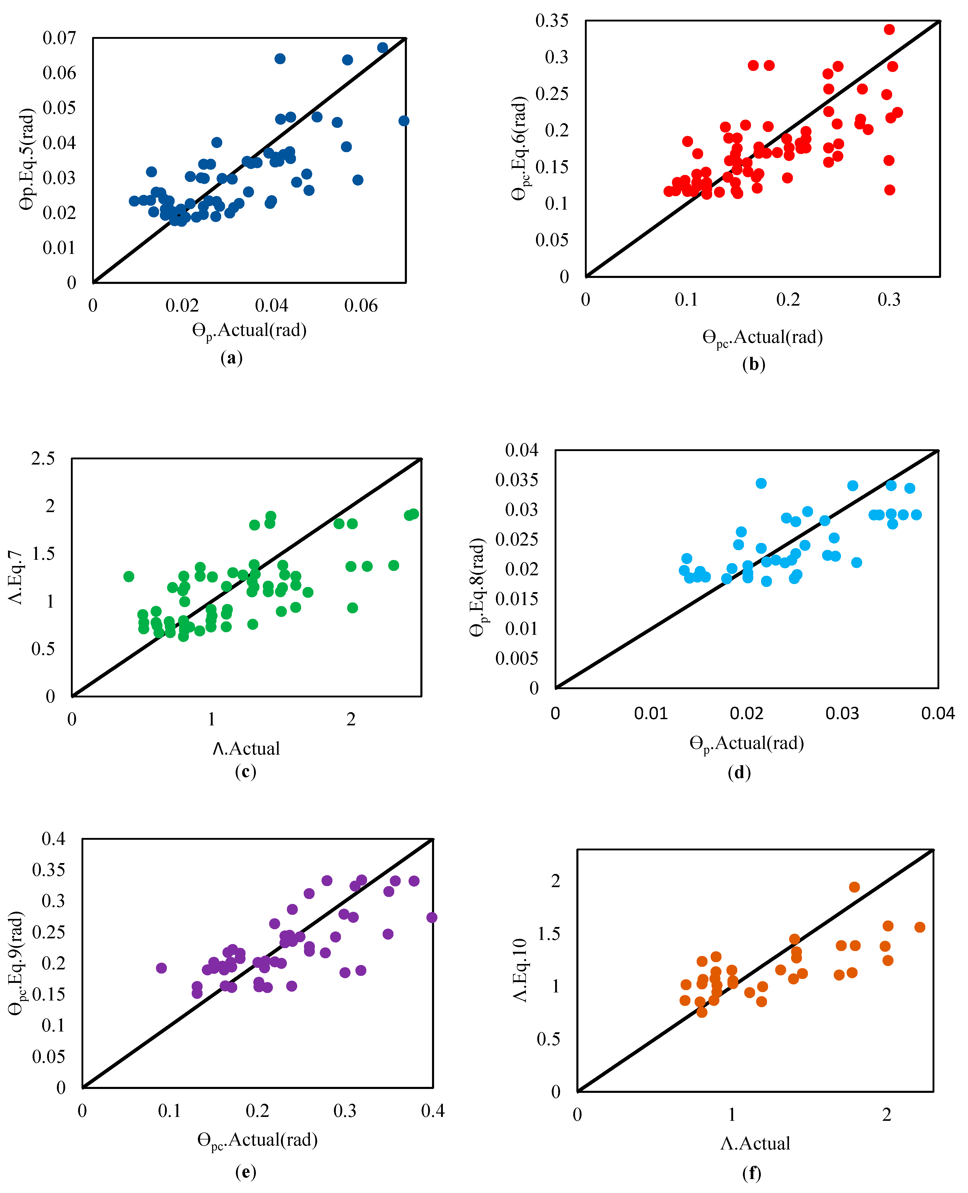
The empirical relationships for obtaining deterioration components in two types of steel beams, referred to as “other than RBS” and “reduced beam section (RBS),” have been developed based on the data obtained from tests [33]. The results from these empirical relationships indicate that for θp, the coefficient of determination (R2) is 0.49 with a root-mean-square error (RMSE) of 0.01 in the “other than RBS” mode, and R2 is 0.47 with an RMSE of 0.0051 in the “with RBS” mode. Furthermore, for θpc, the R2 value is 0.4 with an RMSE of 0.051 in the “other than RBS” mode, and R2 is 0.51 with an RMSE of 0.049 in the “with RBS” mode. Lastly, for Λ, the R2 value is 0.43 with an RMSE of 0.38 in the “other than RBS” mode, and R2 is 0.502 with an RMSE of 0.33 in the “with RBS” mode. A summary of these results is presented in Figure 4.
This study has employed machine learning methods to achieve more accurate predictions of the deterioration components. The following sections elaborate on these findings.
6.2. Base Learners Prediction Results
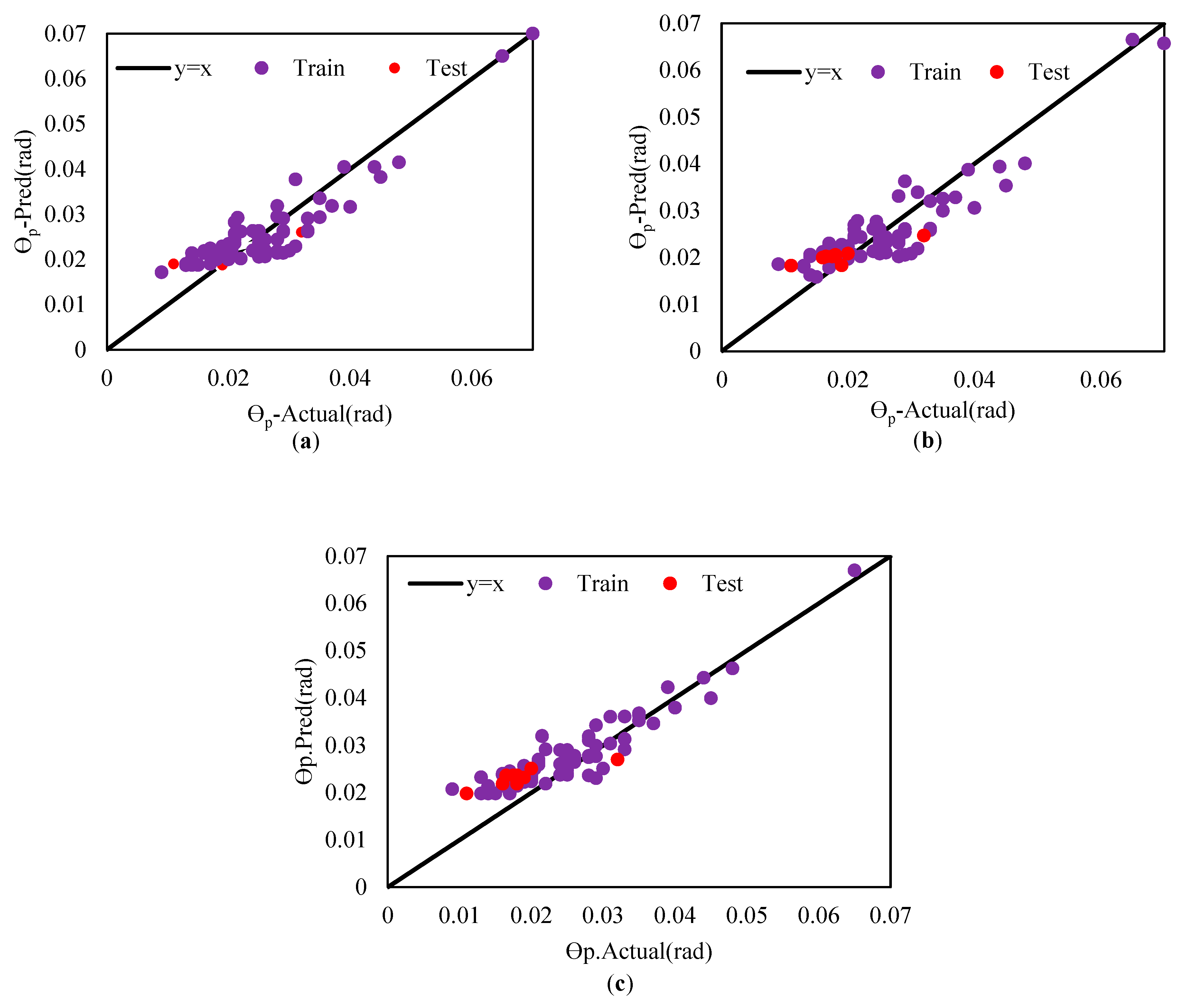
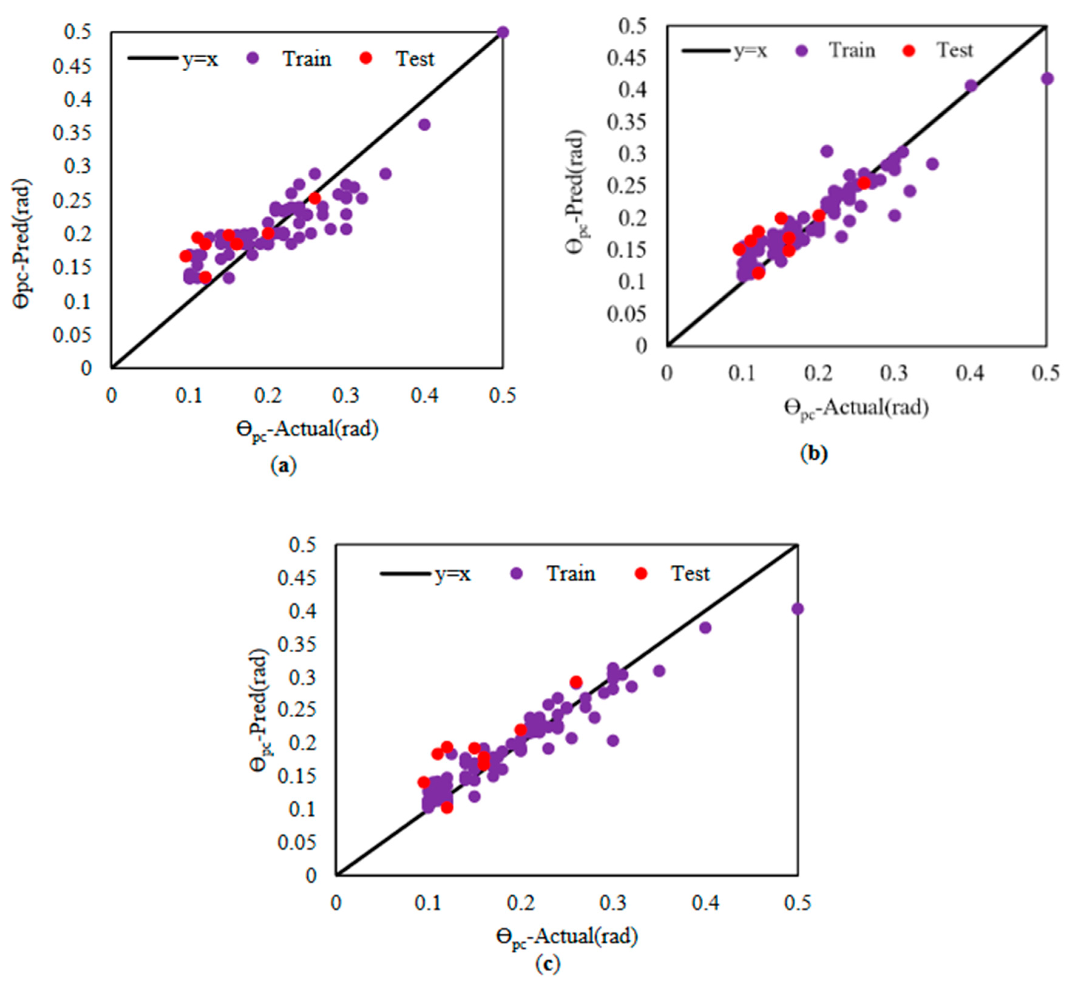
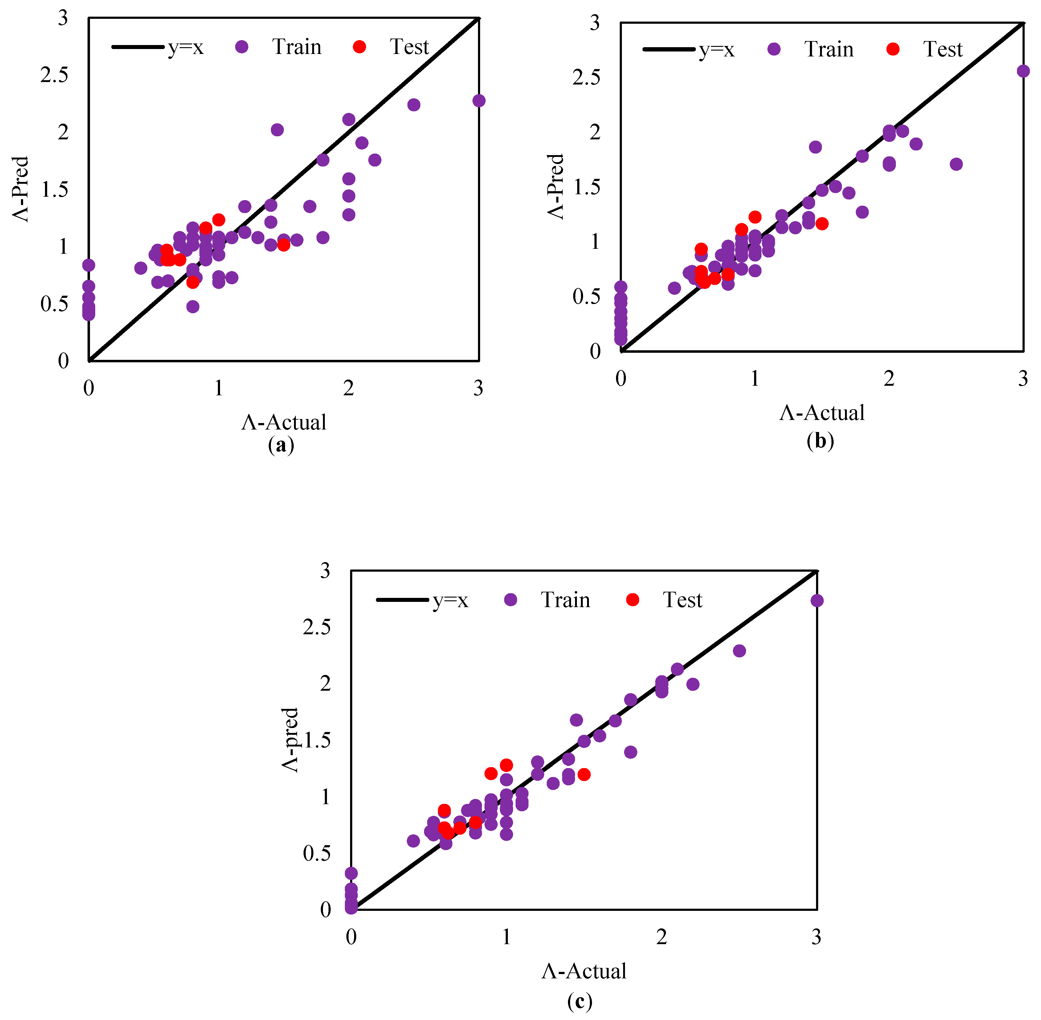
To ensure that the characteristics of the base learners affect the stacking model, the performance of these base learners is evaluated for prediction on both the train and test datasets. The hyperparameters are optimized using a combination of 5-fold cross-validation and grid search. The coefficient of determination (R2) is chosen as the primary evaluation metric. Figure 5, Figure 6 and Figure 7 present the results obtained from the base learners for the train and test datasets, specifically for θp, θpc, and Λ. Further details of the results can be found in Table 4, Table 5 and Table 6. For this research, the base learners selected are AdaBoost, Random Forest, and XGBoost. These learners are utilized as the foundation on which the stacking model is built to enhance the prediction performance.
6.3. Stacking Model Prediction Results
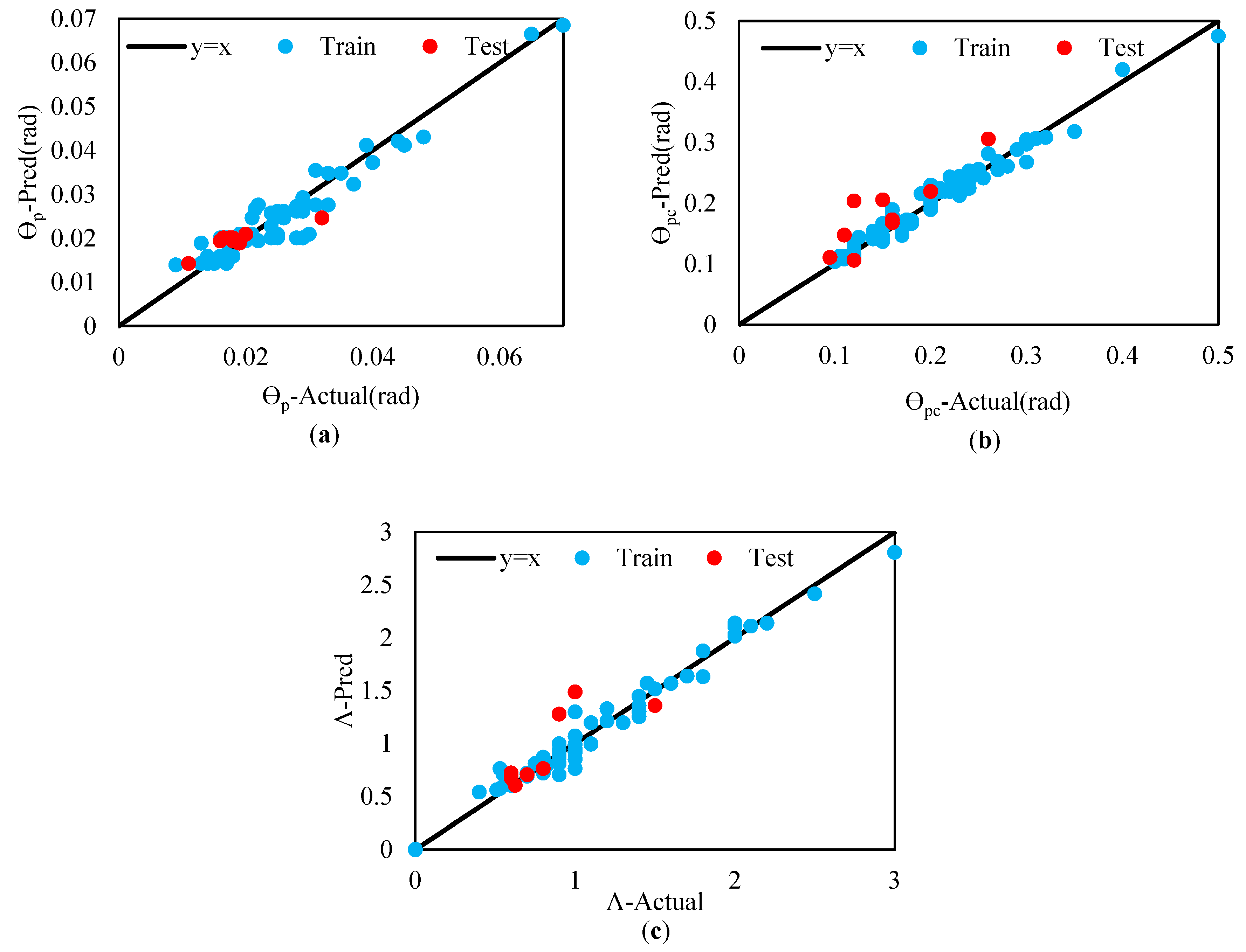
In accordance with Section 6.2, AdaBoost, Random Forest, and XGBoost are chosen as the base learners for the stacking model, with Random Forest being designated as the meta-learner. The prediction results obtained from the stacking model are presented in Figure 8. The stacking model’s predictions for the deterioration components based on the train and test datasets are as follows: For θp, the R2 value is 0.9 with an RMSE of 0.003 for the train data and an R2 of 0.81 with an RMSE of 0.0032 for the test data. For θpc, the R2 is 0.97 with an RMSE of 0.012 for the train data and an R2 of 0.77 with an RMSE of 0.04 for the test data. Finally, for Λ, the R2 is 0.98 with an RMSE of 0.09 for the train data and an R2 of 0.64 with an RMSE of 0.22 for the test data. A comparative analysis of the three models, i.e., base learners, empirical relationships, and stacking, reveals that the stacking model exhibits superior performance and greater accuracy compared to the other models. Detailed results are shown in Figure 9, Figure 10 and Figure 11.
6.4. Comparison of the DCs Models with the Stacking Model
This section evaluates the prediction performance of the proposed model against the experimental model. Mathematical relationships proposed for predicting deterioration components are presented in Equations (5)–(10). Notably, all predictions are within the range of y = x. The stacking model exhibits a significant improvement in R2 and RMSE contrasted to the analytical models. The comparative performance of the stacking model with the analytical models is as follows: For θp, the R2 values were 45.56% and 47.78%, and the RMSE values were 98.52% and 41.18% for the other than RBS and with RBS modes, respectively. For θpc, the R2 values were 58.76% and 47.42%, and the RMSE values were 76.47% and 75.51% for the other than RBS and with RBS modes, respectively. For Λ, the R2 values were 56.12% and 48.78%, and the RMSE values were 76.32% and 72.73% for the other than RBS and with RBS modes, respectively. The results are summarized in Table 4, Table 5 and Table 6.
6.5. Feature Importance Analysis
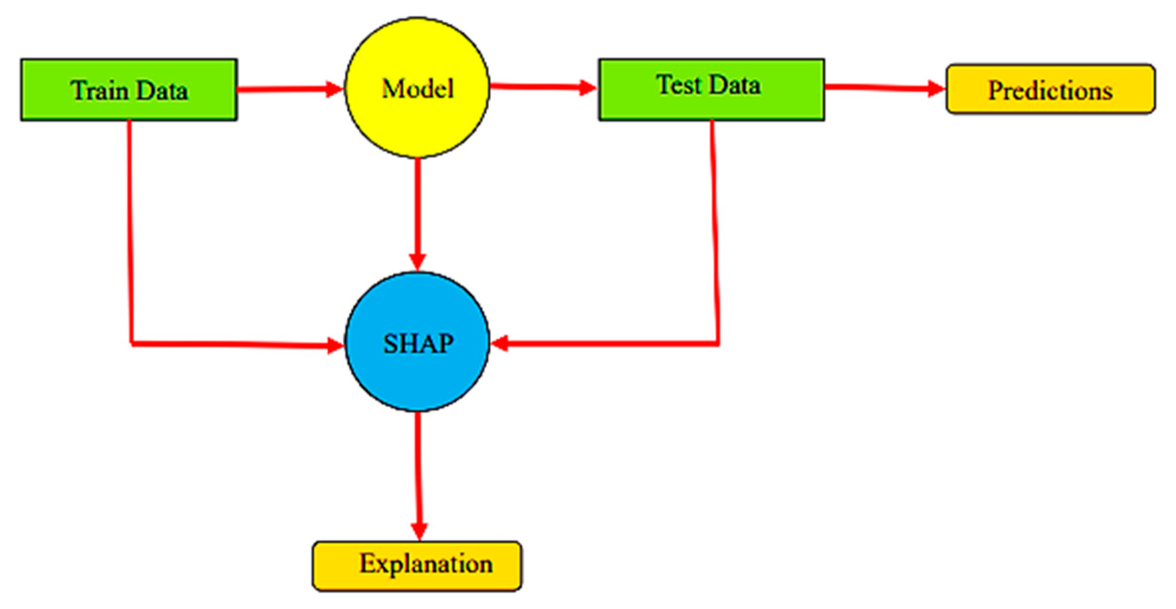
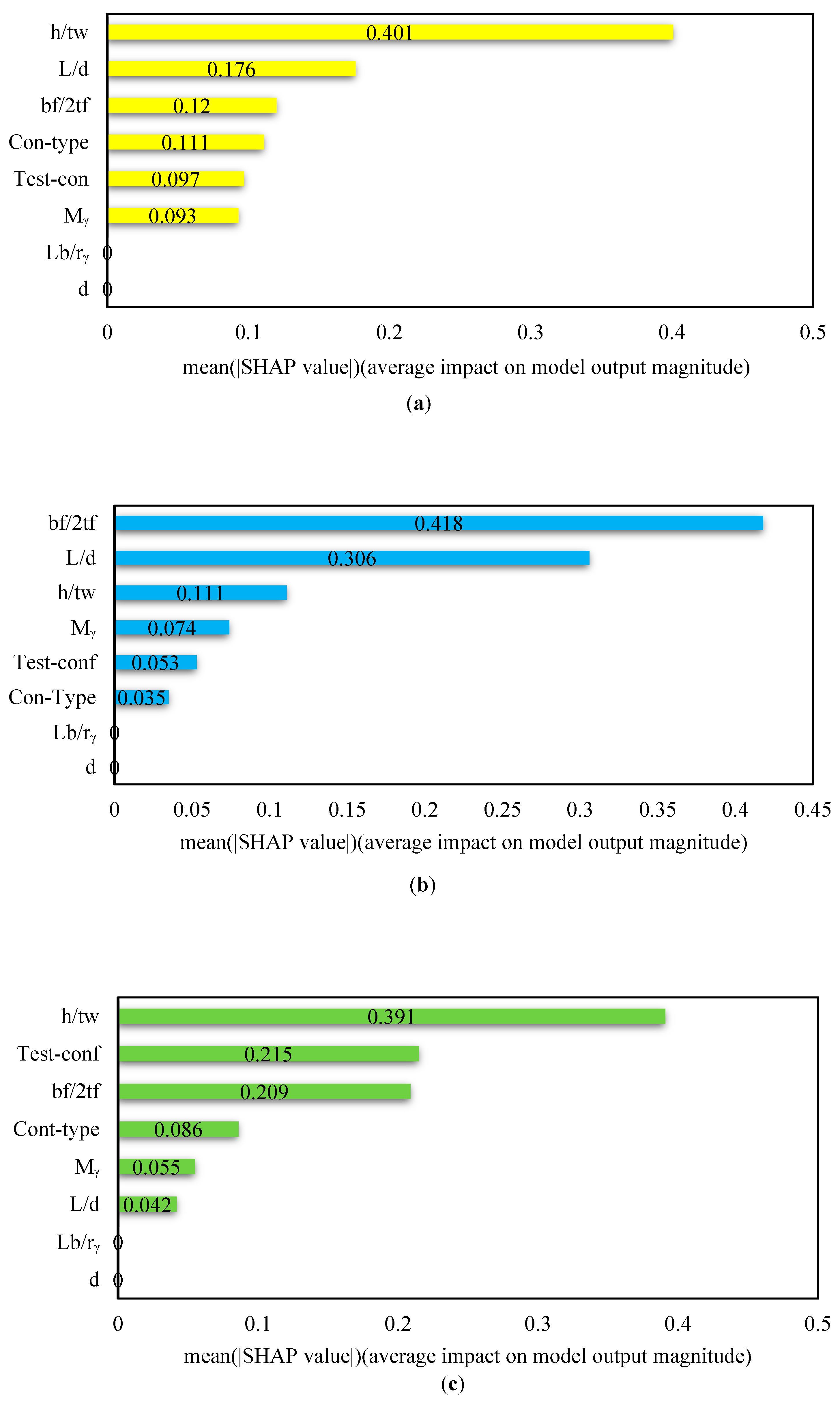
The feature importance indicates their contribution to the model’s prediction. Basically, it determines the usefulness of a particular variable for a current and forecast model. Typically, importance is represented by a numerical score, where a higher score corresponds to greater significance. Feature importance scores offer several benefits. They help establish the relationship between independent variables (attributes) and dependent variables (objectives). By analyzing the importance scores of variables, irrelevant features can be identified and removed. This reduction of irrelevant variables in the model may enhance its performance and speed up computations. Further, feature importance performs as a means for interpreting machine learning models. In this section, we evaluate the importance of variable characteristics using the SHapley Additive exPlanations (SHAP) model. SHAP is a versatile method that can interpret any machine learning model, elucidating the impact of each feature on the target. The SHAP method generates a weighted linear model that assigns Shapley values to different features. Features with higher Shapley values bear more influence on the model’s results, while those with lower values are less influential [41].
The schematic representation of the SHAP method is shown in Figure 12.
The significance of each input variable is computed as a Shapley value, which can be positive or negative depending on the impact on the output.
The basic explanation model function, g(x′), can be defined as:
where x′ is the simplified input variables in vector format acquired from input variables, M is the number of features in the set, φ0 =, and φi denotes the attribution value of each variable. Additive feature attribution methods comprise three desirable properties in the form of local accuracy, messiness, and consistency. A unique explanation to the explanation model g(x′) can be obtained if all three properties are constrained. The explanation model can be expressed as:
where z′∈x′ represents z′ is a subset of x′ and (z′\i) denotes z′i = 0.
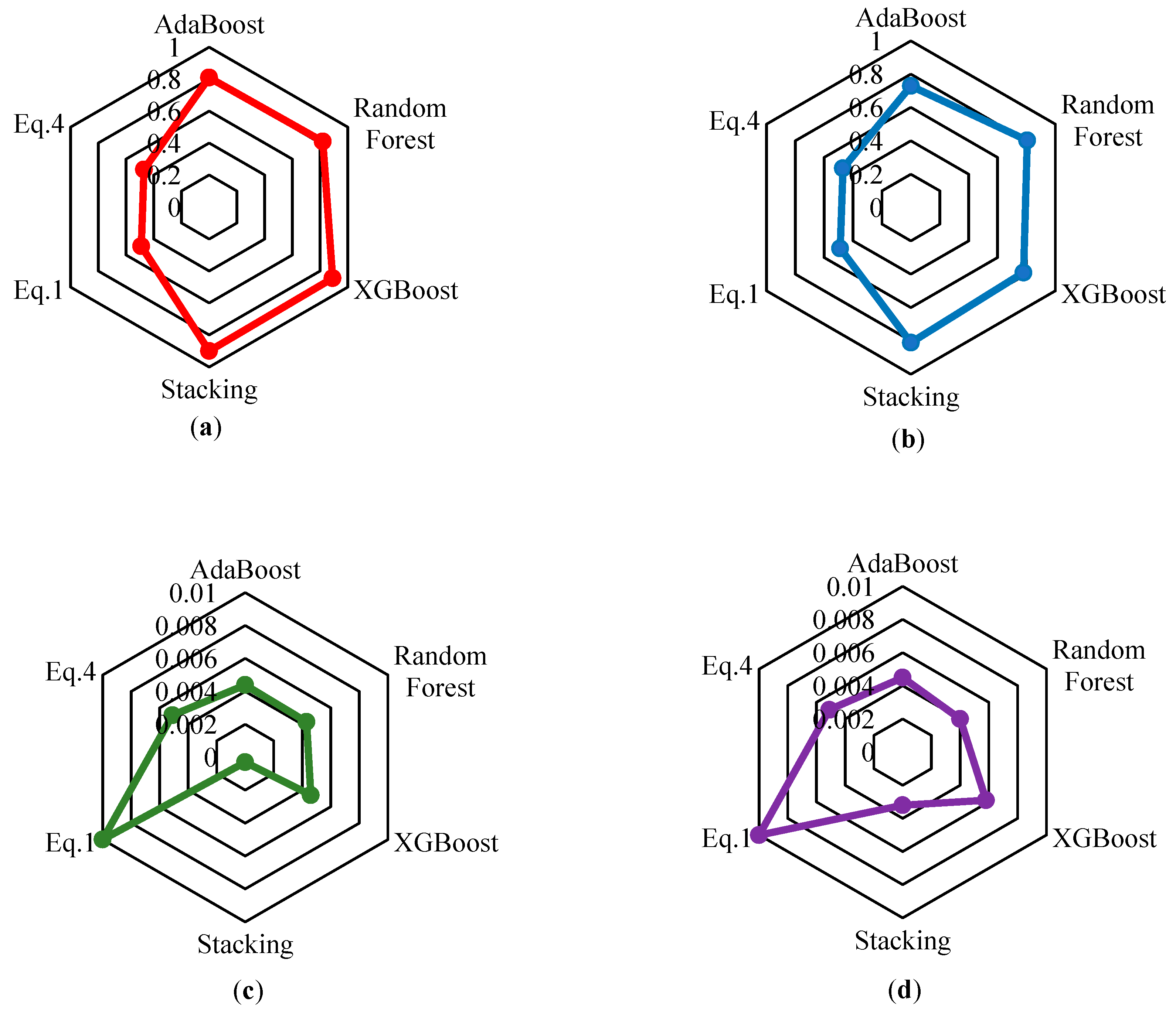
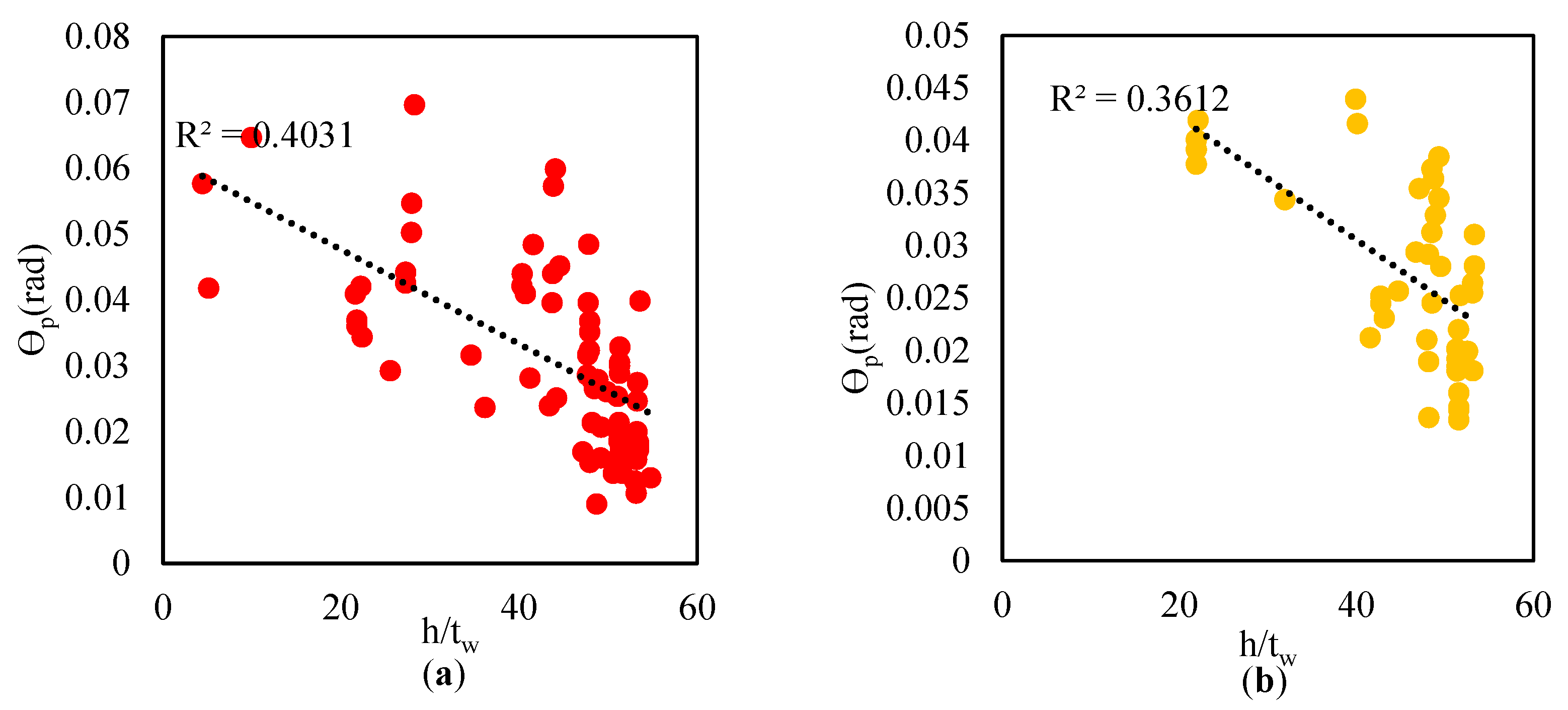
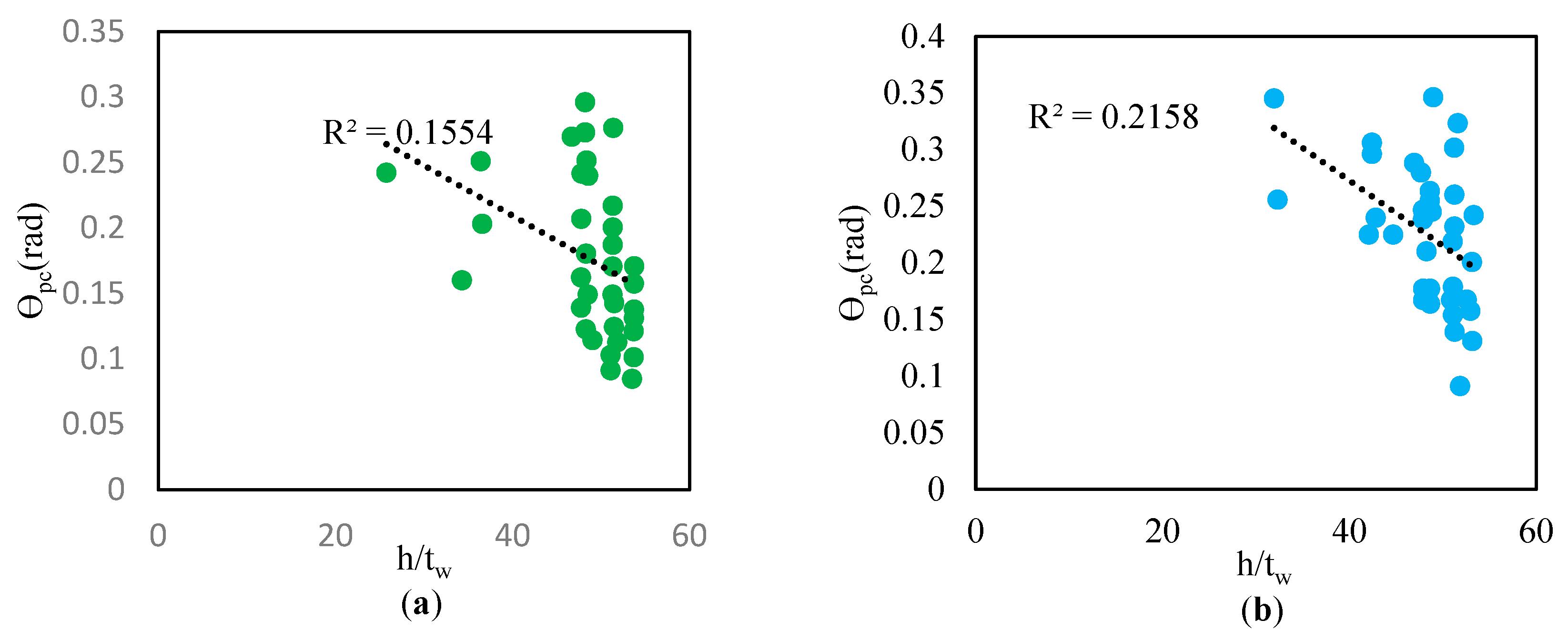
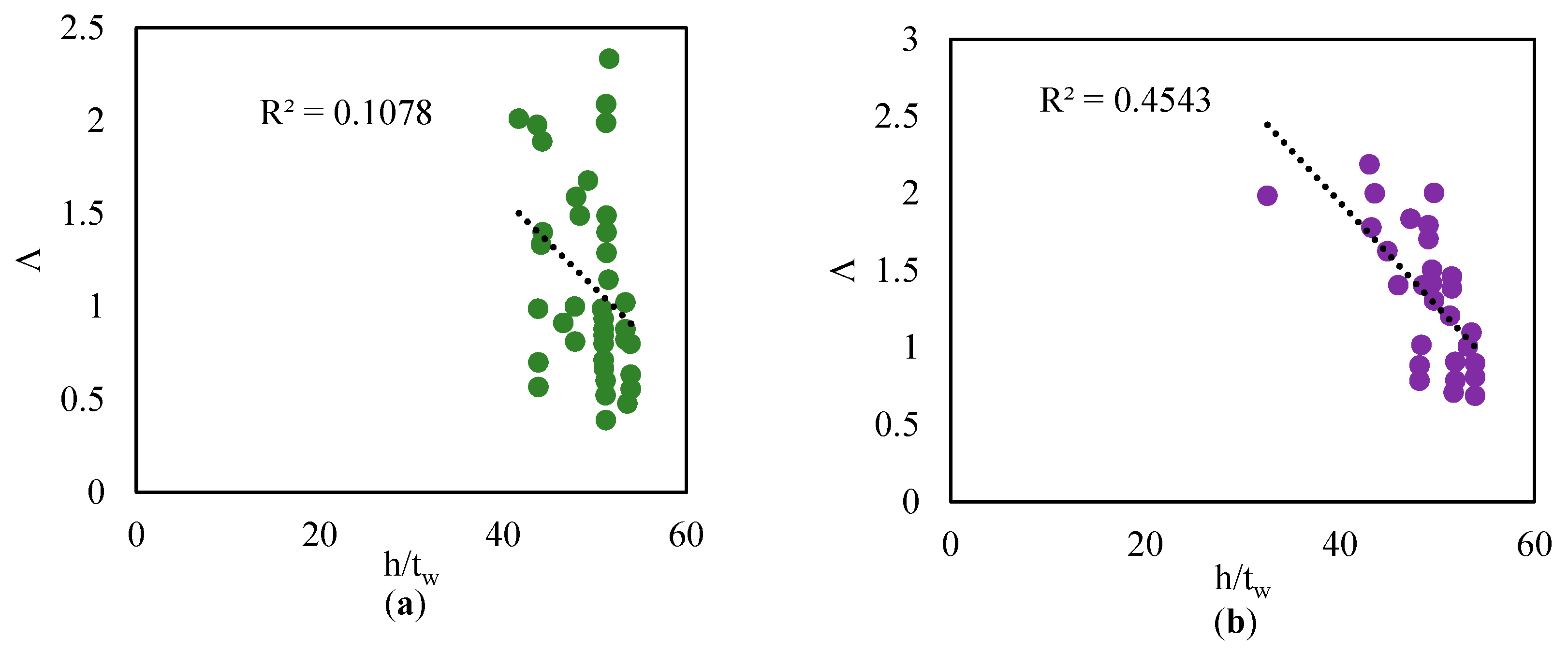
The equation is computationally rigorous due to the multiple possibilities of the subsets of features. Thus, different approximation methods, such as KernalSHAP and TreeSHAP, were proposed to compute the Shapley value. In this study, TreeSHAP was adapted. Shapley values of each input variable were obtained based on the XGBoost model predictions. The analysis reveals that the primary inputs influencing the deterioration components of steel beams are h/tw for θp, bf/2tf for θpc, and h/tw for Λ. Also, the experimental results show that h/tw has the greatest impact in determining the components of deterioration [40] which are illustrated in Figure 13, Figure 14 and Figure 15. On the other hand, in the sensitivity analysis performed by the SHAP, the analysis showed that h/tw and bf/2tf parameters have the most impact. These results are displayed in Figure 16.
7. Conclusions
This study employed the stacking method to predict the deterioration of components of steel beams. The investigation dealt with the performance assessment of both base learners and meta-learners. The stacking model was compared with key machine learning models and analytical relationships related to the deterioration components. Additionally, the importance of input variables was evaluated using the Shapley Additive Explanation model. The stacking model can appropriately merge the prediction outcomes of the base learners and improve the prediction property of the model. The comparison of base learners with the stacking model indicated that the stacking model has high performance compared to other base algorithms. The outstanding findings of this study are summarized as follows:
- The improvements in performance evaluation with the stacking model compared to analytical relationships were as follows:
- For θp, there was a 45.56% increase in R2 and a 98.52% reduction in RMSE for the mode other than RBS, and a 47.78% rise in R2 and a 41.18% decline in RMSE for the mode with RBS.
- For θpc, there was a 58.76% increase in R2 and a 76.47% drop in RMSE for the mode other than RBS, and a 47.42% rise in R2 and a 75.51% decrease in RMSE for the mode with RBS.
- For Λ, there was a 56.12% growth in R2 and a 76.32% decline in RMSE for the mode other than RBS, a 48.78% increase in R2, and a 72.73% reduction in RMSE for the mode with RBS.
- Through a comparative analysis, it was observed that the stacking model outperformed all of the base learners. Furthermore, the stacking model exhibited superior prediction accuracy compared to the AdaBoost, Random Forest, and XGBoost models. The evaluation metrics of the stacking model were as follows: R2 = 0.9 and RMSE = 0.003 for θp, R2 = 0.97 and RMSE = 0.012 for θpc, and R2 = 0.98 and RMSE = 0.09 for Λ.
- Based on the Shapley Additive Explanation model, the variable h/tw (the ratio of web depth to beam web thickness) for θp, the variable bf/2tf (the ratio of flange width to beam flange thickness) for θpc, and the variable h/tw (the ratio of web depth to beam web thickness) for Λ were found to have the most significant impact on determining the deterioration components.
Author Contributions
Investigation, A.K., H.P.S.; software, M.A., A.K.; data curation, A.K., M.A.; formal analysis, A.K.; visualization, A.K.; writing—original draft, A.K.; methodology, H.P.S.; supervision, H.P.S.; resources, H.P.S.; writing—review and editing, H.P.S.; validation, M.A. All authors have read and agreed to the published version of the manuscript.
Funding
This research received no external funding.
Data Availability Statement
The data presented in this study are available on request from the corresponding author (Parvini Sani, H.) upon reasonable request.
Conflicts of Interest
The authors declare that the research was conducted in the absence of any commercial or financial relationships that could be construed as a potential conflict of interest.
References
- Duan, J.; Asteris, P.G.; Nguyen, H.; Bui, X.N.; Moayedi, H. A novel artificial intelligence technique to predict compressive strength of recycled aggregate concrete using ICA-XGBoost model. Eng. Comput. 2021, 37, 3329–3346. [Google Scholar] [CrossRef]
- Thai, H.T. Machine learning for structural engineering. A state-of-the-art review. Structures 2022, 38, 448–491. [Google Scholar] [CrossRef]
- Jayasinghe, T.; Chen, B.W.; Zhang, Z.; Meng, X.; Li, Y.; Gunawadena, T.; Mangaluthu, S.; Mendis, P. Data-driven shear strength predictions of recycled aggregate concrete beams with/without shear reinforcement by applying machine learning approaches. Constr. Build. Mater. 2023, 387, 131604. [Google Scholar] [CrossRef]
- Mangalathu, S.; Jang, H.; Hwang, S.H.; Jean, J.S. Data-driven machine-learning-based seismic failure mode identification of reinforced concrete shear walls. Eng. Struct. 2020, 208, 110331. [Google Scholar] [CrossRef]
- Rahman, J.; Saki Ahmed, K.; Khan, N.L.; Islam, K.; Mangalathu, S. Data-driven shear strength prediction of steel fiber reinforced concrete beams using machine learning approach. Eng. Struct. 2021, 233, 111743. [Google Scholar] [CrossRef]
- Mangalathu, S.; Shin, H.; Chio, E.; Jeom, J.S. Explainable machine learning models for punching shear strength estimation of flat slabs without transverse reinforcement. J. Build. Eng. 2021, 39, 102300. [Google Scholar] [CrossRef]
- Feng, D.C.; Wang, W.J.; Mangalathu, S.; Hu, G.; Wu, T. Implementing ensemble learning methods to predict the shear strength of RC deep beams with/without web reinforcements. Eng. Struct. 2021, 235, 111979. [Google Scholar] [CrossRef]
- Liu, K.; Zou, C.; Zhang, X.; Yan, J. Innovative prediction models for the frost durability of recycled aggregate concrete using soft computing methods. J. Build. Eng. 2021, 34, 101822. [Google Scholar] [CrossRef]
- Hu, G.; Kwok, K.C. Predicting wind pressures around circular cylinders using machine learning techniques. J. Wind Eng. Ind. Aerodyn. 2020, 198, 104099. [Google Scholar] [CrossRef]
- Pyakurel, A.; Dahal, B.K.; Gautam, D. Does machine learning adequately predict earthquake induced landslides? Soil Dyn. Earthq. Eng. 2023, 171, 107994. [Google Scholar] [CrossRef]
- Feng, H.; Miao, Z.; Hu, Q. Study on the uncertainty of machine learning model for earthquake-induced landslide susceptibility Assessment. Remote Sens. 2022, 1, 2968. [Google Scholar] [CrossRef]
- Zhang, C.; Zhu, Z.; Liu, F.; Yang, Y.; Huo, W.; Yang, L. Efficient machine learning method for evaluating compressive strength of cement stabilized soft soil. Constr. Build. Mater. 2023, 392, 131887. [Google Scholar] [CrossRef]
- Asteris, P.G.; Koopialipoor, M.; Armaghani, D.J.; Kotsonis, E.K.; Lourenco, P.B. Prediction of cement-based mortars compressive strength using machine learning techniques. Neural Comput. Appl. 2021, 33, 13089–13121. [Google Scholar] [CrossRef]
- Wang, O.; Al-Tabbaa, A. Preliminary Model Development for Predicting Strength and Stiffness of Cement-Stabilized Soils Using Artificial Neural Networks. In Proceedings of the 2013 ASCE International Workshop on Computing in Civil Engineering, Los Angeles, CA, USA, 23–25 June 2013. [Google Scholar]
- Sayed, Y.A.K.; Ibrahim, A.A.; Tamrazyan, A.G.; Fahmy, M.F.M. Machine-learning-based models versus design-oriented models for predicting the axial compressive load of FRP-confined rectangular RC columns. Eng. Struct. 2023, 285, 116030. [Google Scholar] [CrossRef]
- Nguyen, M.H.; Ly, H.B. Development of machine learning methods to predict the compressive strength of fiber-reinforced self-compacting concrete and sensitivity analysis. Constr. Build. Mater. 2023, 367, 130339. [Google Scholar]
- Chaabene, W.B.; Flah, M.; Nehdi, M.L. Machine learning prediction of mechanical properties of concrete: Critical review. Constr. Build. Mater. 2020, 260, 119889. [Google Scholar] [CrossRef]
- Jiang, K.; Zhao, O. Unified machine-learning-assisted design of stainless steel bolted connections. J. Constr. Steel Res. 2023, 211, 108155. [Google Scholar] [CrossRef]
- Taffese, W.Z.; Espinosa-Leal, L. A machine learning method for predicting the chloride migration coefficient of concrete. Constr. Build. Mater. 2022, 348, 128566. [Google Scholar] [CrossRef]
- Mousavi, M.; Gandomi, A.H.; Hollaway, D.; Berry, A.; Chen, F. Machine learning analysis of features extracted from time–frequency domain of ultrasonic testing results for wood material assessment. Constr. Build. Mater. 2022, 342, 127761. [Google Scholar] [CrossRef]
- Li, H.; Lin, J.; Zhao, D.; Shi, G.; Wu, H.; Wei, T.; Li, D.; Zhang, J. A BFRC compressive strength prediction method via kernel extreme learning machine-genetic algorithm. Constr. Build. Mater. 2022, 344, 128076. [Google Scholar] [CrossRef]
- Sandeep, M.S.; Tipark, K.; Kaewunruen, S.; Pheinsusom, P.; Pansuk, W. Shear strength prediction of reinforced concrete beams using machine learning. Structures 2023, 47, 1196–1211. [Google Scholar] [CrossRef]
- Kaveh, A.; Javadi, S.M.; Moghani, R.M. Shear strength prediction of FRP-reinforced concrete beams using an extreme gradient boosting framework. Period. Polytech. Civ. Eng. 2022, 66, 18–29. [Google Scholar] [CrossRef]
- Lee, S.; Lee, C. Prediction of shear strength of FRP-reinforced concrete flexural members without stirrups using artificial neural networks. Eng. Struct. 2014, 61, 99–112. [Google Scholar] [CrossRef]
- Degtyarev, V.V. Neural networks for predicting shear strength of CFS channels with slotted webs. J. Constr. Steel Res. 2021, 177, 106443. [Google Scholar] [CrossRef]
- Stoffel, M.; Bamer, F.; Markert, B. Artificial neural networks and intelligent finite elements in nonlinear structural mechanics. Thin-Walled Struct. 2018, 131, 102–106. [Google Scholar] [CrossRef]
- Jiang, L.; Tang, Q.; Jiang, Y.; Cao, H.; Xu, Z. Bridge condition deterioration prediction using the whale optimization algorithm and extreme learning machine. Buildings 2021, 13, 2730. [Google Scholar] [CrossRef]
- Hwang, S.H.; Mangalathu, S.; Shin, J.; Jeon, J.S. Machine learning-based approaches for seismic demand and collapse of ductile reinforced concrete building frames. J. Build. Eng. 2021, 34, 101905. [Google Scholar] [CrossRef]
- Farooq, F.; Ahmed, W.; Akbar, A.; Aslam, F.; Alyosef, R. Predictive modeling for sustainable high-performance concrete from industrial wastes: A comparison and optimization of models using ensemble learners. J. Clean. Prod. 2021, 292, 126032. [Google Scholar] [CrossRef]
- Li, S.; Liew, J.R.; Xiong, M.X. Prediction of fire resistance of concrete encased steel composite columns using artificial neural network. Eng. Struct 2021, 245, 112877. [Google Scholar] [CrossRef]
- Li, D.; Cui, S.; Zhang, J. Experimental investigated on reinforcing effects of engineered cementitious composites (ECC) on improving progressive collapse performance of planer frame structure. Constr. Build. Mater. 2022, 347, 128510. [Google Scholar] [CrossRef]
- Li, Q.; Song, Z. Prediction of compressive strength of rice husk ash concrete based on stacking ensemble learning model. J. Clean. Prod. 2023, 382, 135279. [Google Scholar] [CrossRef]
- Lignos, D.G.; Krawinkler, H. Deterioration modeling of steel components in support of collapse prediction of steel moment frames under earthquake loading. J. Struct. Eng. 2011, 137, 1291–1302. [Google Scholar] [CrossRef]
- Livingston, F. Implementation of Breiman’s random forest machine learning algorithm. Mach. Learn. J. Pap. 2005, ECE591Q, 1–13. [Google Scholar]
- Cao, Y.; Qi, G.; Miao, J.; Liu, C.; Cao, L. Advance and prospects of AdaBoost algorithm. Acta Auto. Sin. 2013, 39, 745–758. [Google Scholar] [CrossRef]
- Chen, T.; Guestrin, C. Xgboost: A scalable tree boosting system. In Proceedings of the 22nd ACM SIGKDD International Conference on Knowledge Discovery and Data Mining, San Francisco, CA, USA, 13–17 August 2016; Association for Computing Machinery: New York, NY, USA, 2016. [Google Scholar]
- Sikora, R.; Al-laymoun, O. A Modified Stacking Ensemble Machine Learning Algorithm Using Genetic Algorithms. Int. J. Inf. Technol. Manag. 2014, 23, 1. [Google Scholar] [CrossRef]
- Anguita, D.; Gheladoni, L.; Ghio, A.; Oneto, L.; Ridella, S. The ‘K’ in K-fold Cross Validation. In Proceedings of the 2012 European Symposium on Artificial Neural Networks, Computational Intelligence and Machine Learning, Bruges, Belgium, 25–27 April 2012. [Google Scholar]
- Fu, W.; Nair, V.; Menzies, T. Why is differential evolution better than grid search for tuning defect predictors? arXiv 2016, arXiv:1609.02613. [Google Scholar]
- Lignos, D.; Krawinkler, H. Sidsway Collapse Deterioration Structural Systems under Seismic Excitations; TR 177; The John A. Blume Earthquake Engineering Center: Stanford, CA, USA, 2008. [Google Scholar]
- García, M.V.; Aznarte, J.L. Shapley additive explanations for NO2 forecasting. Ecol. Inform. 2020, 56, 101039. [Google Scholar] [CrossRef]
Figure 1.
Backbone curve definition.

Figure 2.
The stacking ensemble framework.

Figure 3.
Folding data using cross-validation function.

Figure 4.
Predictions of empirical relationships obtained by Lignos and Krawinkler. (a): Equation (5), (b):Equation (6), (c): Equation (7), (d): Equation (8), (e): Equation (9), (f): Equation (10) [33].
Figure 4.
Predictions of empirical relationships obtained by Lignos and Krawinkler. (a): Equation (5), (b):Equation (6), (c): Equation (7), (d): Equation (8), (e): Equation (9), (f): Equation (10) [33].

Figure 5.
Prediction for θp. (a): AdaBoost, (b): Random Forest, (c): XGBoost.

Figure 6.
Prediction for θpc. (a): AdaBoost, (b): Random Forest, (c): XGBoost.

Figure 7.
Prediction for Λ. (a): AdaBoost, (b): Random Forest, (c): XGBoost.

Figure 8.
Prediction based on Stacking for: (a): θp, (b): θpc, (c): Λ.

Figure 9.
Prediction results on the train and test sets for θp, (a):R2-θp-Train, (b): R2-θp-Test, (c):RMSE-θp-Train, (d):RMSE-θp-Test.
Figure 9.
Prediction results on the train and test sets for θp, (a):R2-θp-Train, (b): R2-θp-Test, (c):RMSE-θp-Train, (d):RMSE-θp-Test.

Figure 10.
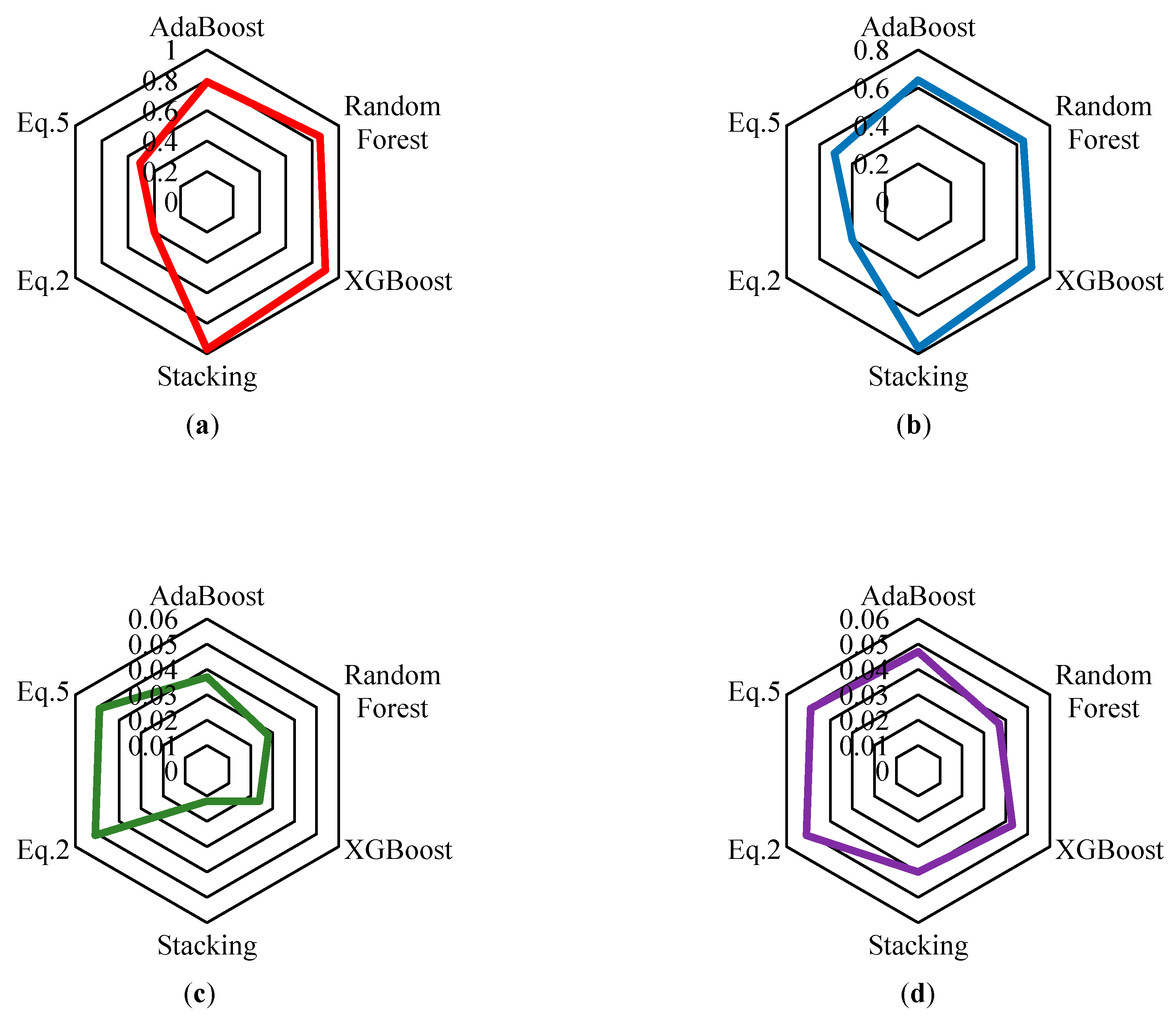
Prediction results on train and test sets for θpc, (a):R2-θpc-Train, (b): R2-θpc-Test, (c):RMSE-θpc-Train, (d):RMSE-θpc-Test.
Figure 10.
Prediction results on train and test sets for θpc, (a):R2-θpc-Train, (b): R2-θpc-Test, (c):RMSE-θpc-Train, (d):RMSE-θpc-Test.

Figure 11.
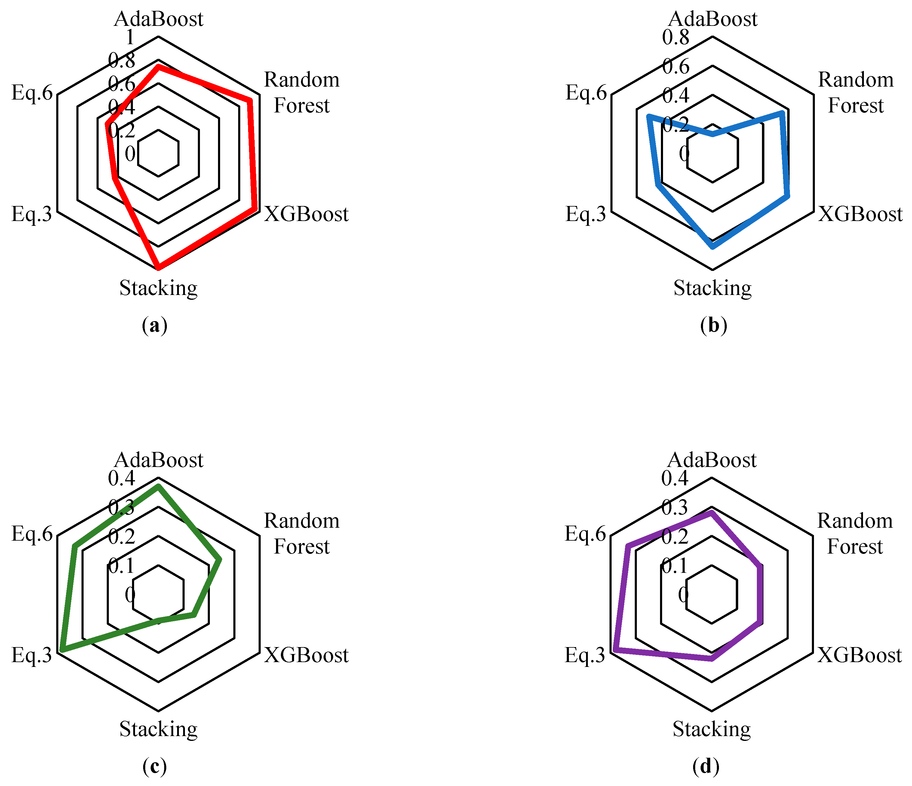
Prediction results on train and test sets for Λ, (a):R2-Λ-Train, (b): R2-Λ-Test, (c):RMSE-Λ-Train, (d):RMSE-Λ-Test.
Figure 11.
Prediction results on train and test sets for Λ, (a):R2-Λ-Train, (b): R2-Λ-Test, (c):RMSE-Λ-Train, (d):RMSE-Λ-Test.

Figure 12.
The schematic representation of the SHAP method.

Figure 13.
Dependence of θp on h/tw for the all data set (data from [40]), (a): other than RBS, (b): with RBS.
Figure 13.
Dependence of θp on h/tw for the all data set (data from [40]), (a): other than RBS, (b): with RBS.

Figure 14.
Dependence of θpc on h/tw for the all data set (data from [40]), (a): other than RBS, (b): with RBS.
Figure 14.
Dependence of θpc on h/tw for the all data set (data from [40]), (a): other than RBS, (b): with RBS.

Figure 15.
Dependence of Λ on h/tw for all datasets (data from [40]), (a): other than RBS, (b): with RBS.
Figure 15.
Dependence of Λ on h/tw for all datasets (data from [40]), (a): other than RBS, (b): with RBS.

Figure 16.
Mean SHAP values of each input parameter in components of deterioration, (a): for θp, (b): for θpc,(c): for Λ.
Figure 16.
Mean SHAP values of each input parameter in components of deterioration, (a): for θp, (b): for θpc,(c): for Λ.


Table 1.
Connection Type (Adapted from [40]).
Table 1.
Connection Type (Adapted from [40]).
| Connection Type |
|---|
| Welded Unreinforced Flanges-Bolted Web |
| Welded Unreinforced Flange-Welded Web |
| Free Flange |
| Reduced Beam Section |
| Bolted Flange Plate |
| Bolted Unstiffened End Plate |
| Bolted Stiffened End Plate |
| Welded Flange Plate |
| Welded Flange Plate-Free Flange |
| Double Split Tee |
| Slotted Web Connection |
| Bolted Bracket Connection |
| Welded Stiffened End Plate |
| Welded Unreinforced Flange-Bolted Web, Welded Plate |
| Ribs-Welded Unreinforced Flange-Bolted Web |
| Bottom Haunch-Welded Unreinforced Flange-Bolted Web |
| Haunches-Welded Unreinforced Flange-Bolted Web |
| Haunches-Bolted Flange-Bolted Web |
| Haunches-Bolted Flange-Bolted Web, Bottom |
| Cover and Side Plate |
| Japanese Welded Unreinforced Flange-Welded Web |
| Japanese Welded-Bolted Web |
| Japanese Welded-Bolted Web-Tapered Flange |
| Korean-T-Stiffener-Welded |
| Extended Tee |
| Extended Tee with Taper |
| Bolted Split-Tee with Shear Tab |
| Bolted Split-Tee without Shear Tab |
| Tee-Bolted |
Table 2.
Test configuration description (adapted from [40]).
Table 2.
Test configuration description (adapted from [40]).
| Test Configuration Description |
|---|
| Standard, single beam, no slab |
| Standard, two beams, no slab |
| Non-Standard-1, column end fixed, single beam, no slab |
| Non-Standard-1, column end fixed, two beams, no slab |
| Non-standard-2, single beams, no slab |
| Non-standard-2, two beams, no slab |
| Non-standard-3, column stub, single beam, no slab |
| Double curvature assembly |
Table 3.
Description of the input and output parameters.
| Describe of Column | Parameter | Unit |
|---|---|---|
| the web-depth-over-web-thickness ratio | h/tw | |
| the flange width-to-thickness ratio used for compactness | bf/2tf | |
| the shear span-to-depth ratio of the beam | L/d | |
| the beam depth of the cross section | d | in |
| the ratio between beam unbraced length Lb over radius of gyration | Lb/ry | |
| Yield moment | My | Kips-in |
| Connection type | Con-type | |
| Test configuration | Test-conf | |
| pre-capping plastic rotation | θp | rad |
| post-capping plastic | θpc | rad |
| cumulative rotation capacity | Λ |
Table 4.
Prediction performance of the stacking model versus existing empirical model for θp.
| Regression Method | Training Set | |
|---|---|---|
| R2 | RMSE | |
| Equation (5) | 0.49 | 0.203 |
| Equation (8) | 0.47 | 0.0051 |
| Stacking | 0.9 | 0.003 |
| Improvement Equation (5) (%) | 45.56 | 98.52 |
| Improvement Equation (8) (%) | 47.78 | 41.18 |
Table 5.
Prediction performance of the stacking model versus existing empirical model for θpc.
| Regression Method | Training Set | |
|---|---|---|
| R2 | RMSE | |
| Equation (6) | 0.4 | 0.051 |
| Equation (9) | 0.51 | 0.049 |
| Stacking | 0.97 | 0.012 |
| Improvement Equation (6) (%) | 58.76 | 76.47 |
| Improvement Equation (9) (%) | 47.42 | 75.51 |
Table 6.
Prediction performance of the stacking model versus existing empirical model for Λ.
| Regression Method | Training Set | |
|---|---|---|
| R2 | RMSE | |
| Equation (7) | 0.43 | 0.38 |
| Equation (10) | 0.502 | 0.33 |
| Stacking | 0.98 | 0.09 |
| Improvement Equation (7) (%) | 56.12 | 76.32 |
| Improvement Equation (10) (%) | 48.78 | 72.73 |
Disclaimer/Publisher’s Note: The statements, opinions and data contained in all publications are solely those of the individual author(s) and contributor(s) and not of MDPI and/or the editor(s). MDPI and/or the editor(s) disclaim responsibility for any injury to people or property resulting from any ideas, methods, instructions or products referred to in the content. |
© 2024 by the authors. Licensee MDPI, Basel, Switzerland. This article is an open access article distributed under the terms and conditions of the Creative Commons Attribution (CC BY) license (https://creativecommons.org/licenses/by/4.0/).
Share and Cite
MDPI and ACS Style
Khoshkroodi, A.; Parvini Sani, H.; Aajami, M. Stacking Ensemble-Based Machine Learning Model for Predicting Deterioration Components of Steel W-Section Beams. Buildings 2024, 14, 240. https://doi.org/10.3390/buildings14010240
AMA Style
Khoshkroodi A, Parvini Sani H, Aajami M. Stacking Ensemble-Based Machine Learning Model for Predicting Deterioration Components of Steel W-Section Beams. Buildings. 2024; 14(1):240. https://doi.org/10.3390/buildings14010240
Chicago/Turabian StyleKhoshkroodi, A., H. Parvini Sani, and M. Aajami. 2024. "Stacking Ensemble-Based Machine Learning Model for Predicting Deterioration Components of Steel W-Section Beams" Buildings 14, no. 1: 240. https://doi.org/10.3390/buildings14010240
Note that from the first issue of 2016, this journal uses article numbers instead of page numbers. See further details here.
Article Metrics
Article metric data becomes available approximately 24 hours after publication online.