
Neural Network Algorithm with Reinforcement Learning for Microgrid Techno-Economic Optimization


Electrical Engineering Department, College of Engineering, Imam Mohammad Ibn Saud Islamic University, Riyadh 11564, Saudi Arabia
Mathematics 2024, 12(2), 280; https://doi.org/10.3390/math12020280
Submission received: 13 December 2023
/
Revised: 4 January 2024
/
Accepted: 12 January 2024
/
Published: 15 January 2024
(This article belongs to the Special Issue Modeling, Optimization and Algorithms for Power Systems)
Abstract
:Hybrid energy systems (HESs) are gaining prominence as a practical solution for powering remote and rural areas, overcoming limitations of conventional energy generation methods, and offering a blend of technical and economic benefits. This study focuses on optimizing the sizes of an autonomous microgrid/HES in the Kingdom of Saudi Arabia, incorporating solar photovoltaic energy, wind turbine generators, batteries, and a diesel generator. The innovative reinforcement learning neural network algorithm (RLNNA) is applied to minimize the annualized system cost (ASC) and enhance system reliability, utilizing hourly wind speed, solar irradiance, and load behavior data throughout the year. This study validates RLNNA against five other metaheuristic/soft-computing approaches, demonstrating RLNNA’s superior performance in achieving the lowest ASC at USD 1,219,744. This outperforms SDO and PSO, which yield an ASC of USD 1,222,098.2, and MRFO, resulting in an ASC of USD 1,222,098.4, while maintaining a loss of power supply probability (LPSP) of 0%. RLNNA exhibits faster convergence to the global solution than other algorithms, including PSO, MRFO, and SDO, while MRFO, PSO, and SDO show the ability to converge to the optimal global solution. This study concludes by emphasizing RLNNA’s effectiveness in optimizing HES sizing, contributing valuable insights for off-grid energy systems in remote regions.
1. Introduction
Many countries worldwide have shown interest in renewable energy conversion sources such as wind and solar photovoltaic (PV) due to the limited lifespan of fossil fuels, which is projected to be only a few more decades. Furthermore, around three billion individuals reside in geographically isolated and rural areas across the globe [1]. Remote areas lacking access to the grid are categorized as off-grid loads. The inherent uncertainty associated with renewable energy sources poses substantial challenges, making reliance on a single renewable energy conversion resource particularly difficult for the electrification of rural loads [2]. Hybrid energy systems (HESs) integrate several power resources, including solar photovoltaic (PV) modules/panels, wind turbine generators (WTs), diesel generators, fuel cells (FCs), and batteries. Hybrid energy systems offer a viable and dependable alternative for providing electricity to off-grid and distant locations. Additionally, they can help delay or eliminate the expenses associated with extending the power grid. HES sizing and design offer an extremely complex nonlinear optimization challenge, despite their numerous benefits, such as environmental friendliness, reduced storage needs, and low maintenance costs [3]. The optimal size of HESs is crucial for obtaining techno-economic benefits since they not only contribute to energy or cost reduction but also extend their functional lifespan [4]. Moreover, optimal sizing refers to a complex optimization design challenge that seeks to minimize one or several objectives while adhering to certain constraints. Efficient energy storage solutions pose an ongoing challenge in HES design [5]. The need to store surplus energy captured during peak times for use during low-generation periods requires identifying suitable and cost-effective energy storage technologies. Furthermore, balancing the economic aspects of HES design is a crucial challenge, considering the initial costs of components, long-term benefits, and operational costs. Ensuring the economic viability of HESs is vital for widespread adoption and sustained success. Moreover, community engagement and acceptance are critical, especially in off-grid and remote areas [6]. Designing HESs that align with local needs, preferences, and socioeconomic conditions is essential for garnering support and ensuring long-term sustainability.
Hence, the primary step to resolve this issue aims to identify the objective function of the system design, whereas the second crucial step aims to select the appropriate optimizer that will be used to address this problem, with the aim of designing microgrid/HES elements based on the predetermined objective function [7]. Currently, the process of determining the optimal sizing of HES components often involves transforming it into an optimization problem. Optimization problems may be solved using two distinct approaches: deterministic techniques and metaheuristic methods [8]. Due to the nonlinear nature and complicated objective functions involved in selecting the components of an HES, deterministic methods are seldom utilized to tackle these optimization issues because of the following factors [9]. Initially, these approaches are highly sensitive to the initial solutions, which can rapidly become stuck in the local optima. Furthermore, these strategies rely on rigorous mathematical assumptions and may be in need of gradient information. In contrast to deterministic approaches, metaheuristic approaches use simplicity and unpredictability to emulate natural processes. For instance, the particle swarm optimizer (PSO) is motivated by social behavior of bird swarming [10], whereas cuckoo search (CS) is motivated by the brood parasitism observed in some cuckoo species [11]. Metaheuristic approaches are more suited for addressing difficult optimization issues compared to deterministic methods due to their simplicity and unpredictability. Several metaheuristic techniques have been utilized to determine the appropriate size of HESs with different technical and/or economic objectives [12,13]. The technical objectives are primarily focused around assessing the reliability of the HES using various reliability parameters, including loss of load expected (LOLE), loss of power supply probability (LPSP), loss of energy expected (LOEE), loss of load hours (LOLH), deficiency of power supply probability (DPSP), equivalent loss factor (ELF), unmet load (UL), and renewable energy fraction (REF). The life cycle cost (LCC), cost of energy (COE), net present cost (NPC), and annualized system cost (ASC) are all included in the economic goals.
Table 1 provides an overview of the reviewed literature for this study. This table summarizes a diverse collection of research endeavors focused on optimizing HES configurations, each employing distinct methodologies and addressing unique technical objectives. In the realm of photovoltaic (PV) and diesel hybrid systems [14,15], the application of the Harmony Search (HS) algorithm aims at minimizing both the annualized system cost (ASC) and carbon dioxide (CO2) emissions, showcasing a dual emphasis on economic and environmental sustainability. The Grey Wolf Optimizer (GWO) [15] was applied to optimize the annualized system cost (ASC) by including PV panels, WTs, and battery storage. This algorithm considers power balancing limitations and focuses on maintaining equilibrium between power generation and consumption. The authors in [16] introduced the Firefly Algorithm (FA) to address the conflicting objectives of minimizing the cost of energy (COE) and mitigating load dissatisfaction, offering insights into balancing economic efficiency and consumer satisfaction in hybrid energy systems. The inclusion of Artificial Bee Swarm Optimization (ABS) in the PV/WTs/FC configuration [17] underscores a focus on minimizing ASC with adherence to the loss of power supply probability (LPSP). Similarly, studies incorporating the Genetic Algorithms (GAs) approach [7,18,19] tackle challenges such as ASC minimization, LPSP constraints, and reducing CO2 emissions, showcasing the versatility of GA in optimizing various aspects of hybrid systems. The particle swarm optimizer (PSO) is prevalent in optimizing PV/WTs/battery [20], PV/WTs/FC [21], and PV/wind/diesel/FC/battery [22] configurations. These studies delve into multi-objective optimization, considering factors such as unsupplied load (UL), net present cost (NPC), and CO2 emissions. Additionally, a comparative analysis was conducted in [23] involving Tabu Search (TS), Simulated Annealing (SA), PSO, and HS, emphasizing PSO’s superior performance in ASC minimization. Furthermore, hybrid approaches, such as combining GA with PSO [24] and utilizing the CS algorithm alongside GA and PSO [2], demonstrate the potential synergies in optimizing NPC and LPSP. The integration of the Mine Blast Algorithm (MBA) [25] introduces a novel perspective in ASC minimization for PV/WTs/FC systems, showcasing its efficiency and reliability compared to other metaheuristic techniques. Studies involving the Crow Search Algorithm (CSA) [26,27] emphasize minimizing NPC while considering constraints like Energy Loss Fraction (ELF) and COE. Additionally, the Improved Firefly Algorithm (IFA) [28] addresses ASC and CO2 emissions in a PV/WTs/diesel/battery configuration. The introduction of the Flower Pollination Algorithm (FPA) in PV/WTs/FC [29] prioritizes minimizing NPC, LOLE, and LOEE, providing a holistic view of system performance. The inclusion of the Grasshopper Optimization Algorithm (GOA) in PV/WTs/battery/diesel [30] explores the optimization of COE and DPSP, underlining the significance of addressing economic considerations and system reliability.
The Multi-objective Line-up Competition Algorithm (MLUCA) stands out for its adeptness in simultaneously minimizing greenhouse gas (GHG) emissions and total annual cost (TAC) in PV/WT/diesel/battery systems [38]. Ant Colony Optimization (ACO) emerges as a noteworthy contender, excelling in TAC minimization across configurations involving photovoltaic technology, wind turbine generators, diesel generators, and battery banks [39]. The Mine Blast Algorithm (MBA) showcases versatility by effectively addressing TAC reduction in PV/WT/diesel/FC/hydrogen tank systems [40]. The Preference-Inspired Co-Evolutionary Algorithm (PICEA) exhibits proficiency in simultaneously minimizing Annual Cost of Supply (ACS), LPSP, and fuel emissions in PV/WT/diesel/battery configurations [41]. Hybrid Grey Wolf with Cuckoo Search Optimization (GWCSO) is applied to determine the optimal size of solar PV, WT, biomass gasifiers, batteries, and a standby diesel generator based on the total annualized cost minimization [42]. The application of the Improved Escaping-Bird Search Algorithm (IEBSA) is employed to ascertain the optimal design for solar PV, WT, and batteries [43]. This optimization is based on the criteria of minimizing energy losses, optimizing the voltage profile, considering the associated system costs, and enhancing the Energy-Not-Supplied (ENS) index [43]. Harris Hawk optimization (HHO) was used to find the best design for the microgrid/HES based on ASC minimization and power network reliability [44]. The Improved Fruit Fly Algorithm (IFFA) demonstrates effectiveness in addressing cost and emissions considerations in PV/WT/diesel/battery systems [28]. Harmony-Search-Based Simulated Annealing (HSSA) emerges as a robust choice for minimizing the life cycle cost within PV/WT/hydrogen/battery systems [45]. Genetic Algorithm particle swarm optimization (GAPSO) garners recognition for its prowess in minimizing total present cost in PV/WT/battery systems [24]. Lastly, a neural network (NN) establishes its efficacy in reducing the potential loss of power supply probability (PLPSP) within PV/WT/battery/utility grid systems [46]. This comprehensive review elucidates the diverse landscape of optimization methodologies, offering valuable insights for scholars and practitioners navigating the intricate domain of HES optimization.
The variety and efficacy of artificial neural networks (ANNs) have been prominently demonstrated in numerous facets of our lives in recent years. The neural network algorithm (NNA), inspired by ANNs, has demonstrated exceptional global search capabilities [47]. However, its slower convergence rate and susceptibility to local minima in addressing nonlinear complex optimization problems have prompted further enhancements. This article presents the application of a new variant of NNA known as the reinforcement learning neural network algorithm (RLNNA) for the optimal sizing of standalone HESs [48]. RLNNA introduces key improvements to address NNA’s limitations. First, leveraging the principles of reinforcement learning, a modification factor adjustment approach is proposed to maintain the RLNNA population diversity. Additionally, the incorporation of a historical population in the transfer operator enhances the algorithm’s global search ability. A feedback operator containing both historical and present feedback terms is designed to accelerate convergence. The main contributions can be summarized and listed as follows:
- ▪
- This study introduces an innovative soft computing/metaheuristic algorithm, the reinforcement learning neural network algorithm (RLNNA), strategically applied to optimize the annualized system cost (ASC) and enhance overall system reliability in an autonomous microgrid/hybrid energy system (HES). This research, focusing on an off-grid HES in a rural region of Saudi Arabia, integrates diverse energy sources—solar photovoltaic technology, wind turbine generators, batteries, and a diesel generator—demonstrating a comprehensive approach to improving sustainability and efficiency in energy management.
- ▪
- In the validation phase, the proposed RLNNA is rigorously assessed against prominent algorithms such as PSO, GA, SDO, MRFO, and traditional NNA. The optimization criteria encompass minimizing the annualized system cost (ASC), achieving a 0% loss of power supply probability (LPSP), and maximizing the renewable energy fraction (REF), addressing economic, reliability, and sustainability considerations within the microgrid/HES framework.
- ▪
- Remarkably, RLNNA surpasses the other five AI techniques in convergence time and global solution capture, positioning it as a promising and effective algorithm for optimization challenges within computational intelligence-based algorithms. Conversely, GA and NNA face challenges with local solutions and prolonged convergence times, potentially becoming trapped in local optima.
- ▪
- In conclusion, the study underscores RLNNA’s efficacy in optimizing HES sizing, offering unparalleled performance relative to established soft-computing algorithms. These findings provide valuable insights for researchers and practitioners seeking efficient solutions for off-grid energy systems, particularly in remote locales.
The subsequent sections of this paper are thoughtfully organized to provide a comprehensive exploration of the research. Section 2 serves as an introduction to the site description and meteorological data, establishing the contextual foundation for this study. It describes the proposed HES configuration, shedding light on the details of the system design. This section discusses the integration of various energy sources, storage components, and the overall architecture aimed at fulfilling the energy demands of the off-grid rural area. Section 3 introduces the essential components of the optimization algorithm, specifically the RLNNA, which has been proposed for the optimal sizing of the microgrid/HES. This section elaborates on the unique features and mechanisms of RLNNA in tackling the challenges associated with HES optimization. Section 4 transitions into a detailed discussion of the simulation results. Finally, Section 5 provides the major conclusions drawn from this research.
2. System Description and Mathematical Modeling
2.1. System Description
The methodology applied in this paper encompasses several essential facets crucial to comprehensively understanding and optimizing the HES. The resource data, load profile, control techniques, and system component requirements are all covered in detail in this part.
2.1.1. Meteorological Data
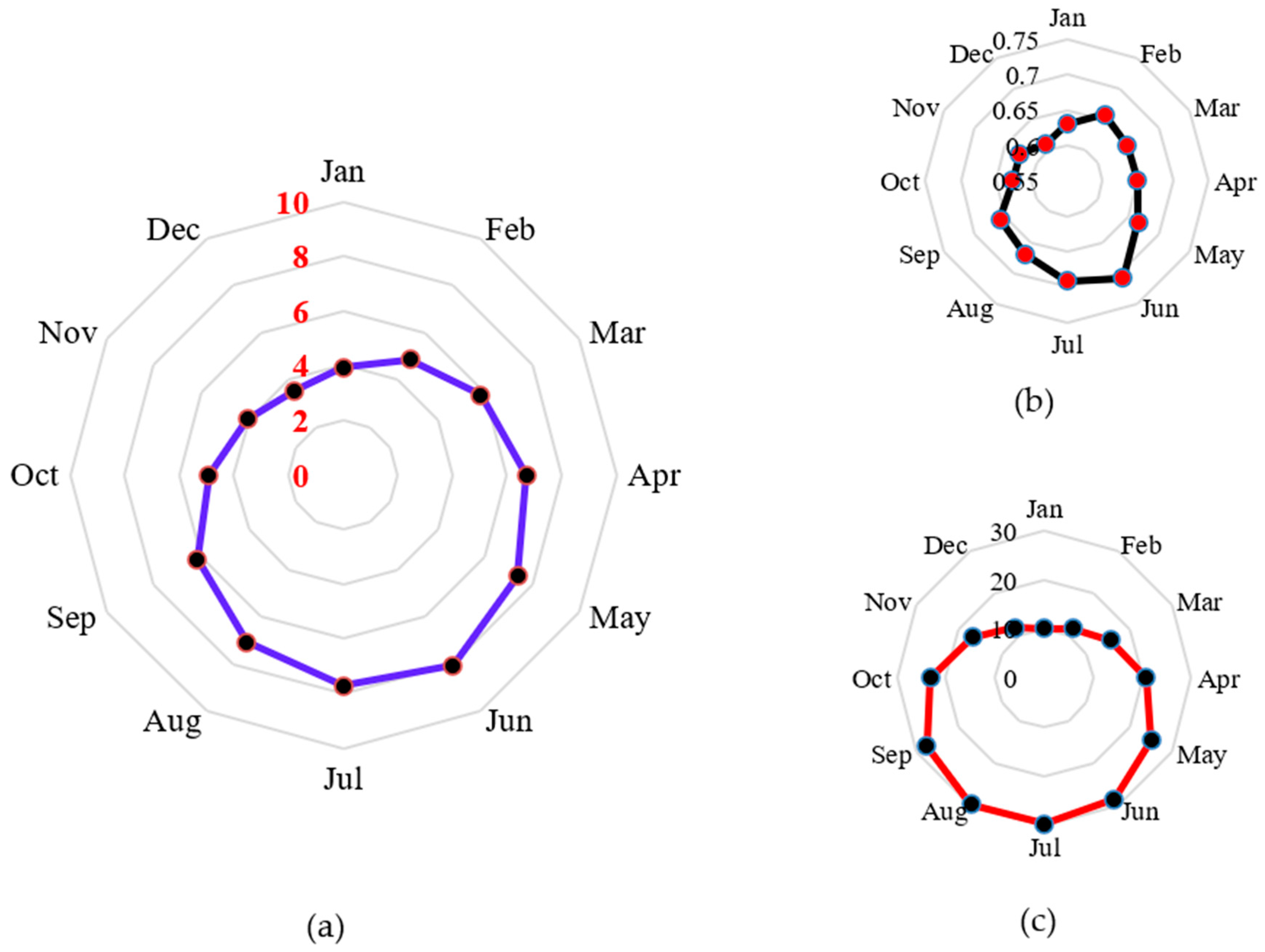
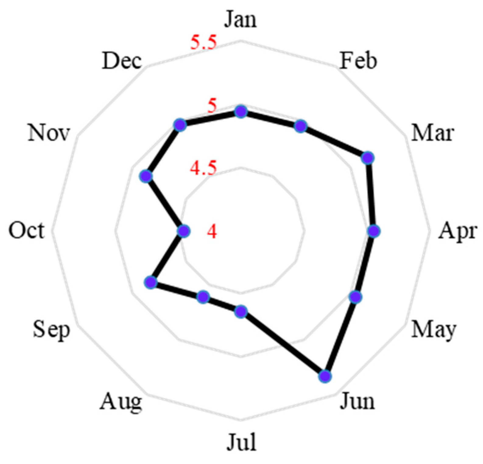
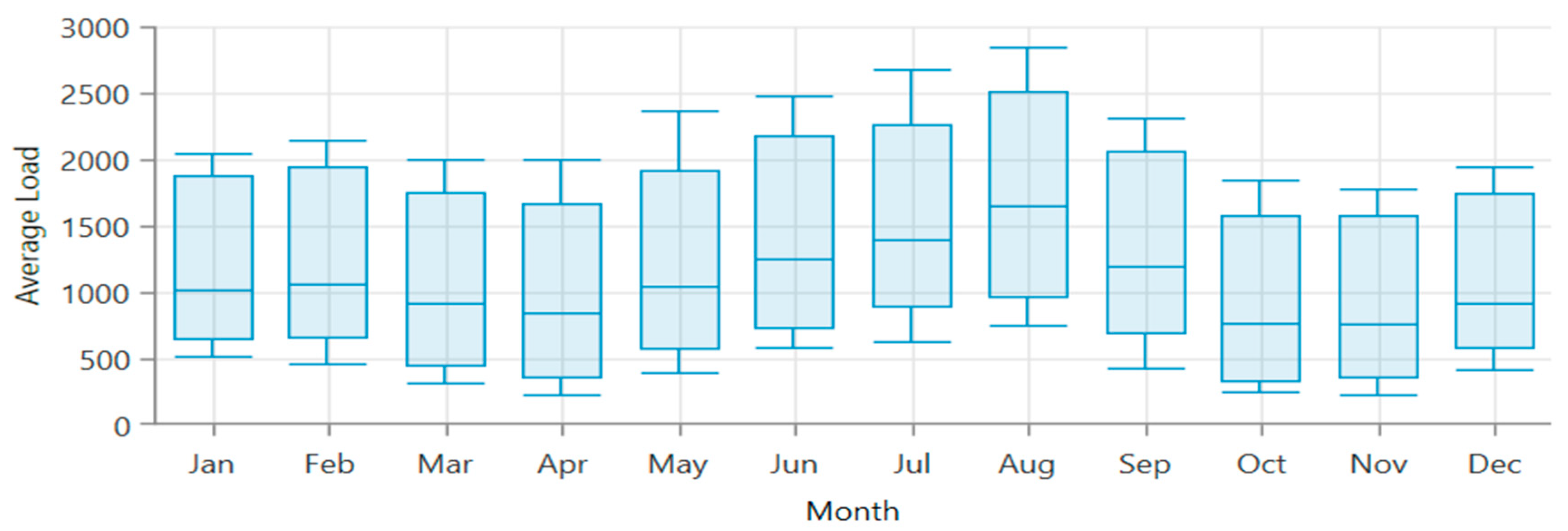
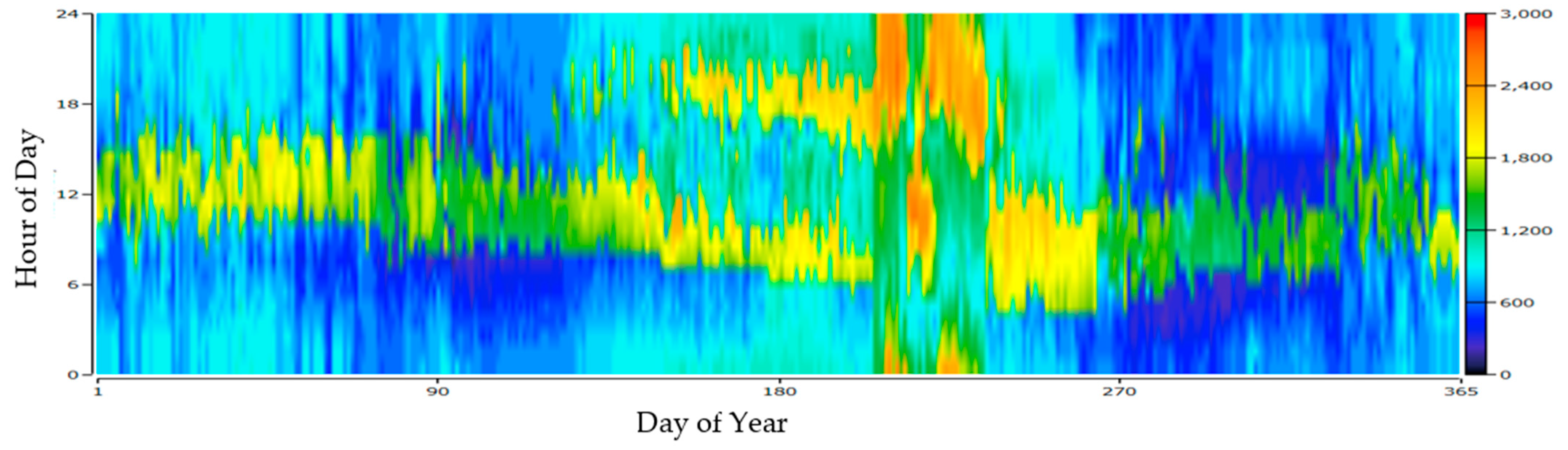
Figure 1 presents a visual representation of the solar irradiance levels and monthly mean temperature on a horizontal surface of the area under study. The monthly wind speed is presented in Figure 2. Notably, the highest and lowest temperature and sun irradiance levels are observed during July and January and June and December, respectively. The generation of hydrogen for industrial uses and the use of electrical loads constitute the city’s energy consumption. Figure 3 illustrates the hourly variation in the load, showcasing the fluctuations in energy demand over the course of a day. Additionally, Figure 4 provides insight into the monthly load variations, demonstrating the changes in energy requirements throughout the months.
These visual representations offer a comprehensive understanding of the climatic conditions and energy consumption patterns within the area under study, which are fundamental factors influencing the design and optimization of the HES for this region. The selected load profile sample, depicted in Figure 3 and Figure 4, is chosen for its high variability in daily energy consumption. This diversity in load variations serves to test the system’s performance across a spectrum of electricity consumption levels. A minimum load demand of 210 kW is suggested, while a peak load demand of 2850 kW is created. The average electricity consumption is estimated at approximately 1070.1 kW. These datasets are critical as they simulate real-world conditions, allowing for comprehensive testing and evaluation of the HES’s performance across varying energy demands and wind conditions.
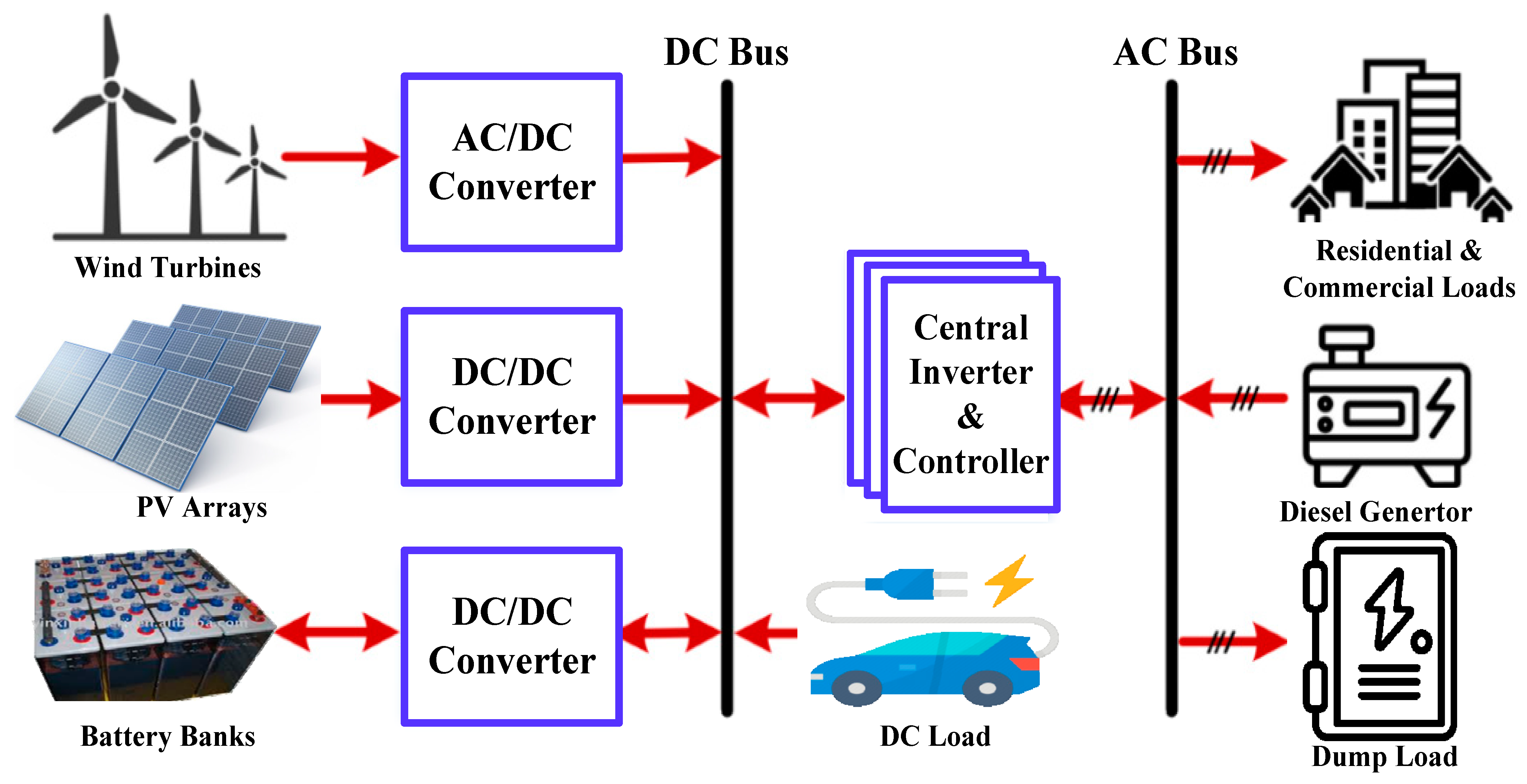
2.1.2. The Microgrid/HES Configuration
The wind turbine, PV system, diesel generator, converter, and batteries are the five main parts of the proposed microgrid/HES. Figure 5 provides a visual representation of the system configuration, offering a schematic illustration of how these components are interconnected and function collectively within the system. Furthermore, the detailed specifications and costs associated with each of these components are outlined in Table 2. This table elucidates the specific characteristics, technical details, and financial costs relevant to the wind turbine, PV system, diesel generator, converter, and batteries integrated within the HES configuration. This comprehensive breakdown is fundamental in understanding the individual contributions of each component to the overall system functionality and economic implications.
2.1.3. The PV/Wind/Diesel/Battery Dispatch Strategy
In HESs, the dispatch strategy plays a pivotal role, acting as a control technique governing the operation of both the battery bank and diesel generator in scenarios where renewable energy sources alone cannot meet the load demand. Optimizing HESs involves performing a techno-economic analysis, and this can be executed through various control techniques, each with distinct advantages and limitations. The proposed technique, developed by MATLAB, aims at offering a more applicable and efficient dispatch technique tailored for microgrid/HESs. This strategy divides its operation into two distinct cases:
Case 1: If the load demand aligns with the power generated from the wind turbines, the wind turbines exclusively supply the load without involving the battery. Consequently, no activation of the generator is required in this scenario.
Case 2: If the power captured by the wind turbines exceeds the load demand, the surplus power is directed towards charging the battery if it is not at full capacity. Should the battery be fully charged, the surplus power is dissipated. Throughout this scenario, the generator remains inactive. However, if the wind power alone cannot meet the load demand, there are further considerations:
- ▪
- If the battery state of charge (SOC) is above the defined minimum SOC (SOCmin), the load requirements are fulfilled through discharging the battery.
- ▪
- If the SOC falls below the minimum threshold (SOCmin), two sub-cases are encountered:
- ✓
- In instances where the load demand falls beneath the minimum load capacity of the diesel generator, the generator functions at its prescribed minimum load ratio. This ratio represents the lowest permissible load on the diesel generator and is typically denoted as a percentage of its overall capacity. For instance, if the stipulated minimum load ratio is established at 40%, and the requisite electrical output from the diesel generator is 50% of its capacity, the diesel generator operates at 50%. Conversely, if the demand is 20%, the generator functions at the minimum load ratio of 40% to avert exceedingly low load operations.
- ✓
- Should the minimum load of the generator be either less than or equivalent to the prevailing load demand, the generator is utilized to fulfil the load requirements without necessitating the involvement of the battery charging process.
The above comprehensive strategy showcases the decision-making process in allocating power from different sources, ensuring optimal utilization while addressing load demand and storage needs within the HES framework.
2.2. Mathematical Modeling
2.2.1. PV System
It is crucial to comprehend the performance of PV systems to accurately estimate their energy output. To compute the hourly output energy of the PV system, critical inputs such as solar irradiance, ambient temperature, and manufacturing information specific to the PV module are utilized within the PV panel. The hourly output power (PPV, module) of the PV panel/module can be estimated using Equation (1) [50]. This equation sums up the relationship between these input factors and the resultant hourly output power generated by the PV panel:
where:
: Represents the rated power of the photovoltaic panel/module, measured in kilowatt (kW). This signifies the power output of the PV array under standard test conditions.
: denotes the photovoltaic derating factor, typically represented as a percentage (%).
: signifies the average solar irradiance incident on the PV array, measured in kW/m2.
: represents the incident irradiation in kW/m2 under standard test conditions.
: stands for the temperature coefficient of power, represented as a percentage change per degree Celsius (%/°C).
: indicates the PV cell temperature, measured in degrees Celsius (°C).
: denotes the temperature of the PV cell under standard test circumstances, expressed in degrees Celsius (°C).
The temperature of a PV module, a critical factor affecting its electrical characteristics, exhibits a strong correlation with environmental conditions. While at night, it aligns with the ambient temperature, but in sunlight, the PV temperature can surpass the ambient temperature by 30 °C or above. As such, estimating the PV module temperature becomes crucial. The steady-state temperature of the PV panel/module can be estimated using Equation (2) [50], which takes into account factors such as the ambient temperature (), the nominal operating cell temperature (NOCT), the solar irradiance at which NOCT is symbolized as (), and the ambient temperature at which NOCT is symbolized as (), as well as maximum power efficiencies under standard test conditions (). This equation aids in determining the PV module’s temperature under different environmental circumstances, ensuring accurate assessments of its performance.
The maximum power point efficiency () is determined by the following formula:
Hence, when the solar irradiance incident on the PV panel’s surface and the PV panel/module temperature are established, the hourly PV output power generated can be computed using Equation (1). This equation facilitates the determination of the PV system’s power output, considering these critical parameters.
2.2.2. Wind Turbine System Model
Three characteristic speeds—cut-in (), rated (), and cutoff ()—as well as rated power () serve as the foundation for wind turbine models. The output power of wind turbines can be estimated using a variety of models, including quadratic, linear, and Weibull parameter-based models. A quadratic model is utilized in this study to approximate the wind turbine output power captured [49]. A wind turbine’s PWT output power captured can be computed as follows:
In cases where data are typically available at standard heights like 10 m or 20 m, estimations for other heights are necessary based on measured wind speeds. One powerful method is the power law, articulated by equation [49]:
Here, represents the measurement height, denotes the hub height at which wind speed is required, and signifies the power law exponent. This formula is instrumental in estimating wind speeds at different heights using available data at specific standard heights.
2.2.3. Modeling of Diesel Generator
The diesel generator functions to cover the load when the collective energy produced from renewable sources (such as PV, wind turbine, and battery) is insufficient to meet the load requirement. The cost of diesel fuel for the generator is computed using the subsequent equation [50]:
Here, represents the hourly fuel consumption in liters per hour (L/h), contingent upon the load characteristics of the diesel generator, formulated as follows [50]:
where:
: the diesel generator’s rated power, measured in kilowatts (kW).
: the power produced by the diesel generator for a specific hour, measured in kilowatts (kW).
: the fuel cost per liter, denoted in USD per litre (USD/L).
Coefficients A and B: these coefficients, representing the fuel curve, are set at A = 0.246 L/kWh and B = 0.0845 L/kWh, respectively.
The fuel consumption of a diesel generator is significantly influenced by both the rated power and the actual generated power. Consequently, it is imperative for the diesel generator to operate within a specific power range, avoiding operation at its minimum setting. Typically, diesel generator manufacturers provide guidance regarding the minimum operating setting. This operational range of the diesel generator is expressed mathematically as follows:
In the context of the proposed HES, an assessment of the total carbon dioxide (CO2) emissions is conducted across the system’s annual operation. This evaluation involves a comparative analysis between the emissions generated by the proposed HES and those stemming from a scenario where the load demand is solely met by a diesel generator. The calculation of the total CO2 emissions resulting from the fuel combustion of the generator involves considering the emission factor of CO2 per kilowatt-hour (kWh) of electricity generated by the diesel generator. For this research, the emission factor is established at 0.699 kg of CO2 emitted per kWh of electricity generated by the generator [51].
2.2.4. Battery Bank Model
Batteries serve as a critical component in the HES due to the sporadic nature of wind and solar power, influenced by varying weather conditions and the time of day. Battery storage is employed to bridge the energy supply–demand mismatch that may arise from these fluctuations. Selecting an appropriate battery size for the microgrid/HES necessitates a comprehensive analysis, considering various factors, including the maximum depth of discharge, temperature effects, nominal battery capacity, and battery lifetime considerations.
In this research, certain battery efficiency parameters are defined: The round-trip efficiency is used to determine the battery’s charge efficiency, while the discharge efficiency is considered as 1. Based on the operational mode of the system (charging or discharging), the state of charge (SOC) of the battery bank can be estimated using the following formulas [50]:
- ▪
- Charging Mode (when energy generation exceeds load demand):
- ▪
- Discharging Mode (when load demand exceeds energy generation):
and : represent the state of charge of the battery at the current time, t, and the previous time (t − 1), respectively.
: denotes the hourly rate of self-discharging, indicating the rate at which the battery loses charge when not in use.
: signifies the total energy captured at time t by the renewable energy sources in the microgrid/HES.
: corresponds to the load demand at time t, i.e., the electricity required by the system at a specific moment.
: represents the efficiency of the inverter used within the HES.
: represents the battery bank’s charging efficiency, indicating how effectively the battery stores and releases energy.
To maintain the battery within safe operating conditions, two key constraints are imposed:
- ▪
- SOC(t) should not fall below a minimum permissible energy level, denoted as . This level ensures that there is always a certain minimum energy reserve within the battery bank.
- ▪
- During the charging process, SOC(t) should not exceed a maximum permissible energy level, designated as . This limit is often equivalent to the nominal capacity of the battery bank (), ensuring that the battery does not become overcharged and damaged.
The relationship between and can be defined as the maximum depth of discharge (DOD). Specifically, is calculated as (1 − DOD), where is the battery bank’s nominal capacity. This relationship helps ensure that the battery operates within the specified range and longevity limits.
2.2.5. System Reliability Model
The LPSP serves as a key metric for evaluating the reliability of power systems within the HES. It seeks to account for the inherent stochastic characteristics of renewable energy sources, which exert a substantial influence on the dynamics of energy production. LPSP is crucial in the design phase to ensure system reliability. The LPSP is based on specific methodologies, summarizing the steps as follows:
- ▪
- Surplus Energy Storage: if the energy production from renewables exceeds the current load demand, the excess energy is stored in the batteries unit, recalculating the state of charge (SOC) based on Equation (9) until it reaches the maximum limit.
- ▪
- Load Demand Exceeds Renewable Generation: When the load demand surpasses the available energy from renewable energy sources, the battery bank is used to make up the difference. In such cases, SOC is recalculated using Equation (10).
At maximum SOC, the charging process halts as managed by the energy management system. The LPSP over a specific period T (typically a year in this context) is determined by the equation [49]:
Power Failure Time (PFT) represents the duration when the load remains unsatisfied due to insufficient power generation from the HES, providing a measure of system reliability in handling energy demands.
2.2.6. Renewable Energy Fraction Model
The REF is a crucial metric used to quantify the proportion of energy delivered to the load that is generated from renewable sources. It elucidates the system’s reliance on renewable energy. The REF is calculated as follows [50]:
Here, denotes the percentage of load served by the diesel generator in kilowatt-hours (kWh). An REF value of 100% indicates a purely renewable energy system, while an REF of 0% signifies a system reliant solely on diesel power. REF values between these extremes reflect the microgrid/HES, representing the proportion of renewable energy integrated into the overall energy supply.
2.2.7. System Economics Model
The cost of energy (COE) is an essential metric for evaluating system cost analysis within an HES. It represents the average cost per kWh of useful electrical energy generated. The COE can be determined using the following formula [49]:
Here, the total annualized cost of the system in USD per year is referred to as the ASC. The term indicates the total electrical load served by the system over the course of a year, measured in kilowatt-hours per year. The annualized system cost (ASC) comprises three main components: the annualized capital cost (), the annualized replacement cost (), and the annualized maintenance cost (), which has been formulated as follows:
The determination of the annualized replacement cost, the annualized capital cost, and the O&M cost is a crucial component for the overall system cost analysis in the HES. These costs are estimated based on the initial capital investments, system lifetime, and the unit costs of the system elements.
The for each system component, including the PV array, wind turbine, battery banks, and diesel generator, can be determined using the formula:
Here, represents the initial capital cost of each component in USD, while the capital recovery factor (CRF) accounts for the system life period in years ().
The is determined by the sum of the product of the total capacity () and the unit cost () for each system component:
The represents the annualized value for all replacement costs incurred throughout the project’s lifetime, and it can be calculated as:
Here, denotes the replacement cost of the component (USD), while the sinking fund factor (SSF) is determined by the system’s lifetime ().
The following details provide comprehensive insights into the economic aspects and expected lifetime of the HES components. The components, including PV modules, wind turbines, battery banks, inverters, and diesel generators, feature initial costs, potential replacement expenses, and operational and maintenance costs, as well as estimated lifespans and interest rates. The photovoltaic modules are originally priced at USD 1000/kW, with a negligible O&M cost of USD 20 per kW, operating over a 20-year lifespan at a 2% interest rate. The wind turbines initially cost USD 1300 per kW, with a potential O&M cost of USD 30.33 per kW. Similarly, the battery banks start at USD 200 per kilowatt-hour (kWh), featuring O&M costs of USD 5 per kWh and operating across a 10-year span. The inverter shows an initial cost of USD 133 per kW, with a 10-year lifespan and a 2% interest rate. The diesel generator is priced at USD 300 per kW, involving an identical replacement cost, an O&M expense of USD 0.012 per kWh, and a 10-year lifespan.
3. The Framework and Implementation of RLNNA
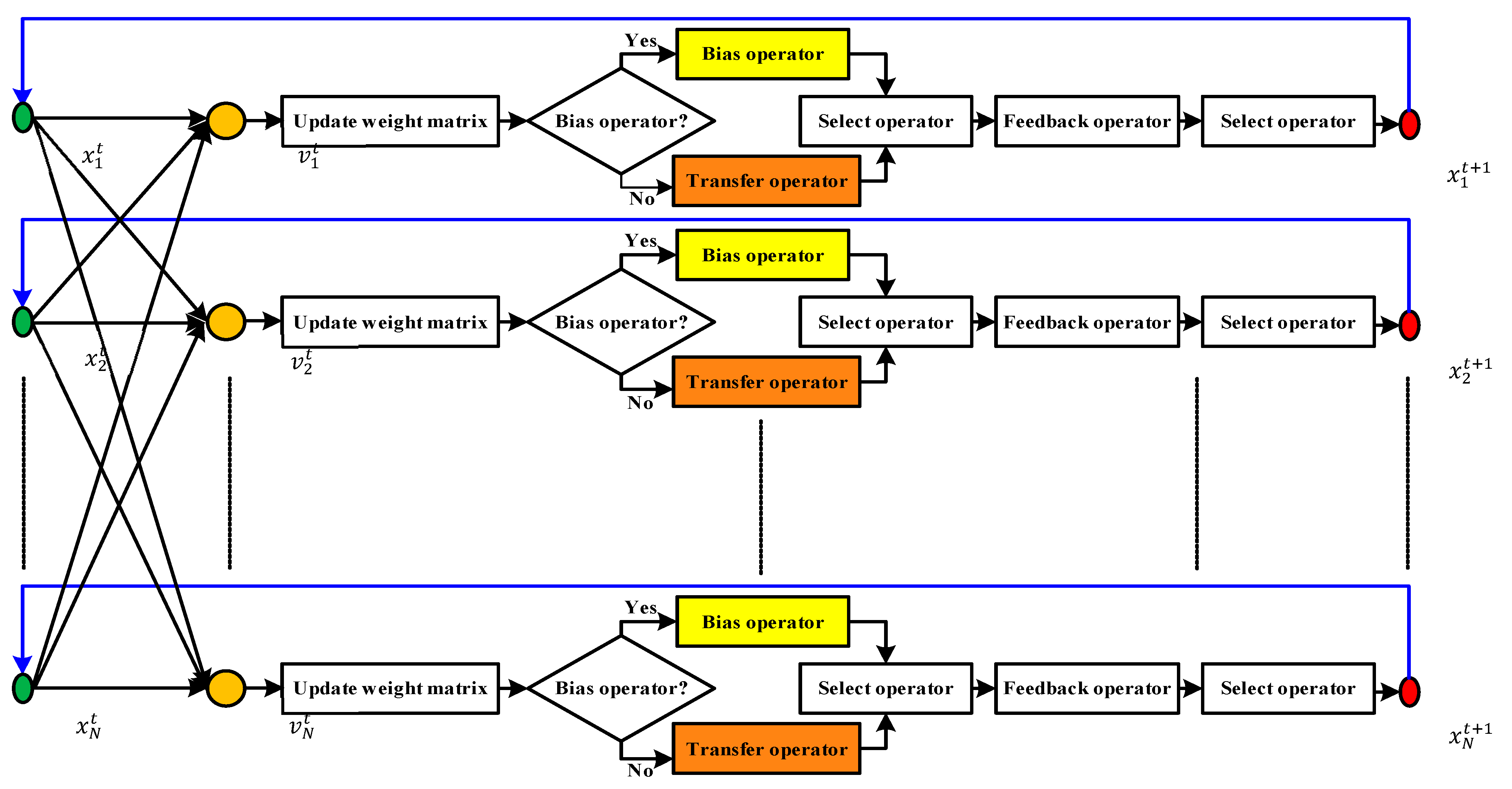
The RLNNA framework encompasses five main phases, as shown in Figure 6, that have been discussed as follows:
3.1. Generating the Trial Population
In RLNNA, the trial population is mathematically formulated as follows:
where N represents the population size, t denotes the current iteration, refers to the ith individual of the population at time t, signifies the ith trial individual of trial population at time t, and represents the jth weight value of the ith individual at time t. The weight matrix complies with the following condition:
3.2. Updating the Weight Matrix
The weight matrix, instrumental in generating the trial population, has been updated by the equation:
where is a random integer number uniformly distributed in the range of 0 to 1, and represents the target weight vector.
3.3. Bias Operator
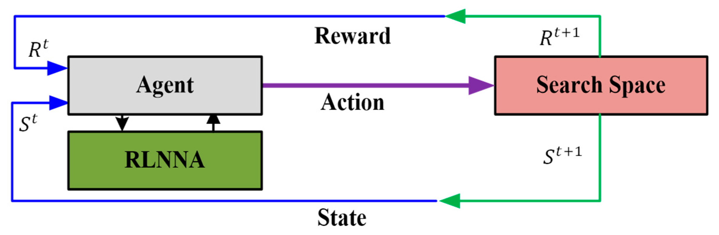
The role of the modification factor, denoted as , within RLNNA is crucial in balancing exploration and exploitation. The principle behind this factor lies in the identification of outstanding individuals, those who secure better solutions within an iteration. These exceptional individuals provide essential insights into approaching the global optimal solution. The strategy is to encourage these outstanding individuals to focus on their vicinity by engaging in a search operator around themselves, which is known as local exploitation. This approach is governed by a designed rule within RLNNA that leverages the fitness values obtained from each individual within an iteration.
where τ represents the penalty factor, and signify two difference functions, and denotes a control function.
, , and can be expressed as:
where represents the fitness value of the ith individual at a given time t. Meanwhile, and denote the fitness values of the ith individual at time t + 1, derived from the first and second function evaluations, respectively. Triggered by this information, two potential actions emerge: the “keep action” and the “activate action”. The “keep action” prompts an individual to maintain the same modification factor used in the previous iteration for their subsequent search. Conversely, the “activate action” instigates the adoption of a new modification factor for the next search. In RLNNA’s dynamic, outstanding individuals—those securing superior solutions within the iteration—will cause the “activate action” to begin. Consequently, their iteration-by-iteration modification factor will decrease, raising the probability that the transfer operator (exploitation) will be executed in the next iteration. A visual representation of the procedure for updating the modification factor is provided in Figure 7.
The bias operator in RLNNA comprises both a bias population and a bias weight matrix. The bias population encompasses a random integer and a set with elements. Variables and show the variables’ lower and upper bounds, respectively, with D being the variables number. Furthermore, equates to (βt × D), and encompasses integer random numbers chosen from 1 to D. One way to express the bias population is as follows:
Here, is a uniformly distributed, randomly generated number between 0 and 1.
Similarly, the bias matrix involves two inputs: a set ϑ comprising elements and a random integer . The definition of the bias weight matrix is:
ξ represents a randomly generated number in the range of 0 to 1.
3.4. Transfer Operator
The transfer operator serves as a mechanism for exploitation within RLNNA, helping to identify superior solutions within the current search space. Comprising a transfer period from the past as well as one from the present, it is represented as:
Here, and are random numbers drawn from a standard normal distribution. The purpose of these random values is to extend the search space, aiding in avoiding local optimal solutions.
The vector represents the ith individual in the historical population at time t, and it is updated according to the following condition:
Here, is uniformly distributed and represents a random integer number in the range of 0 to 1. The final version of is collected by a permuting function, (·), which sorts the vectors randomly.
The population initialization within RLNNA is performed by:
where is a random integer number in the range of 0 to 1, uniformly distributed.
Following the completion of the transfer operator, a selection operator is executed:
3.5. Feedback Operator
The feedback operator, intended to hasten convergence, further optimizes the trial population obtained via the transfer operator:
Here, and are random numbers drawn from the normal distribution. m represents a random integer number in the range of 1 to N, while signifies the mth individual fitness. The feedback operator offers two primary advantages. It takes into consideration the local feedback in addition to current feedback. The strong randomness of the historical feedback term contributes to enhanced population diversity. Finally, following the completion of the feedback operator, a selection operator is executed:
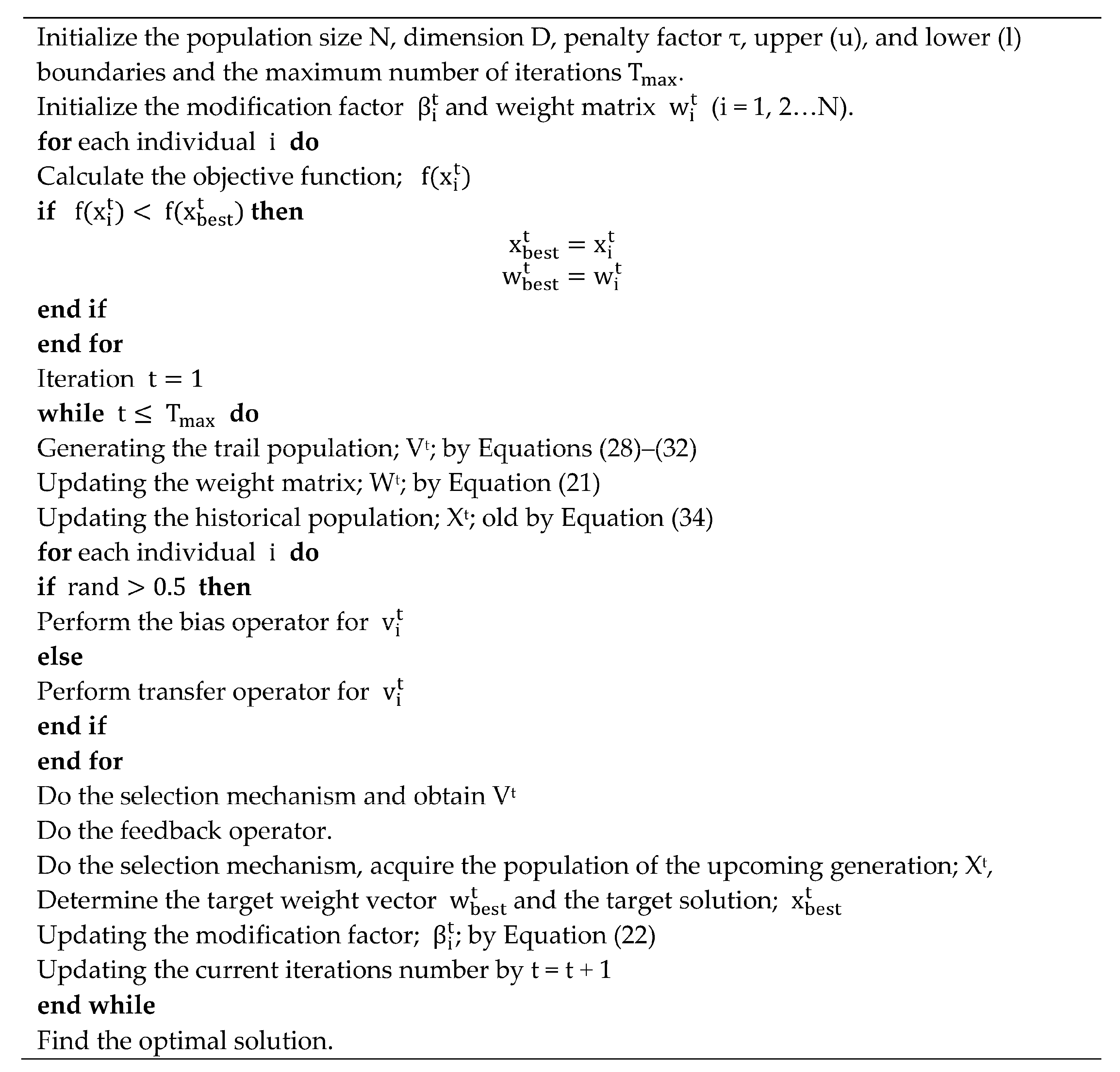
Figure 8 displays the pseudo-code for the RLNNA technique.
4. Simulation Results, Discussion, and Analysis
The RLNNA approach is introduced as a novel technique for optimizing the sizing of a microgrid aimed at supplying a remote region in Saudi Arabia. The proposed RLNNA algorithm leverages the hourly wind speed and solar radiation, offering a unique perspective on HES optimization. The HES under consideration encompasses PV arrays, wind turbine generators (WTs), batteries, and diesel generators, reflecting a comprehensive system design for off-grid energy supply. To assess the performance of the RLNNA algorithm, a thorough comparison was conducted with five contemporary artificial intelligence (AI)-based optimization techniques: GA, PSO, SDO, NNA, and MRFO. The effectiveness of these algorithms was evaluated using four performance indices: the mean, the standard deviation (STD), the optimal/ideal solution, and the worst solution. Key parameters for each algorithm, such as the maximum number of iterations and independent runs number, were standardized at 500 and 50, respectively, for consistency across all evaluations. Table 3 lists the primary characteristics of every AI-based method that was employed in this study. The implementation of all soft-computing algorithms was carried out using MATLAB R2019b on a Windows 10/64-bit platform.
Table 4 shows a comprehensive analysis of six intelligent soft-computing algorithms—GA, PSO, SDO, RLNNA, NNA, and MRFO. For validity purposes, RLNNA was compared to the other five soft-computing algorithms. The focus of this analysis is the optimal sizing of a microgrid/HES required for supplying a residential load in the Kingdom of Saudi Arabia. The concluding remarks collected from this table can be summarized as follows:
- ▪
- RLNNA: Excels with the lowest optimal cost of USD 1,219,744.0, indicating superior performance. While the mean cost of USD 1,221,659.2 is competitive, a slightly higher STD of 112.8 suggests some variability. RLNNA, however, requires a longer elapsed time of 62.9 s.
- ▪
- MRFO: Performs competitively with an optimal cost of USD 1,222,098.4, akin to PSO and SDO. The mean cost of USD 1,222,770.8 demonstrates consistent performance, and the low STD of 1,485.6 signifies reliability. MRFO operates efficiently, with an elapsed time of 44.8 s.
- ▪
- PSO: Yields an optimal cost of USD 1,222,098.2 per year, showcasing effectiveness in HES sizing. The mean cost of USD 1,222,181.4 indicates stability, and the low STD of USD 2,081.2 suggests reliability. PSO demonstrates moderate computational efficiency, with an elapsed time of 41.9 s.
- ▪
- SDO: Mirrors PSO in achieving an optimal cost of USD 1,222,098.2, emphasizing consistent performance. The mean cost of USD 1,222,166.2 and low STD of 68.20 signify reliability in sizing outcomes. SDO exhibits a slightly longer elapsed time of 47.6 s.
- ▪
- NNA: Achieves an optimal cost of USD 1,222,319.5, demonstrating effectiveness in HES sizing. The mean cost of USD 1,224,626.9 suggests stable performance, while a higher STD of 2,388.4 indicates some variability. NNA operates efficiently, with an elapsed time of 27.4 s.
- ▪
- GA: Demonstrates competitive performance with an optimal cost of USD 1,232,654.5 per year. The algorithm exhibits a mean cost of USD 1,247,373.6, indicating consistent performance. However, a relatively high standard deviation (STD) of USD 10,504.0 suggests variability. Notably, GA operates efficiently, with an elapsed time of 27.9 s.
In summary, RLNNA stands out with the lowest optimal cost, while NNA and MRFO demonstrate effectiveness with competitive results and computational efficiency. The choice of algorithm may depend on the specific priorities, such as minimizing costs or achieving a balance between cost optimization and computational speed, in the context of HES design for isolated areas in Saudi Arabia.
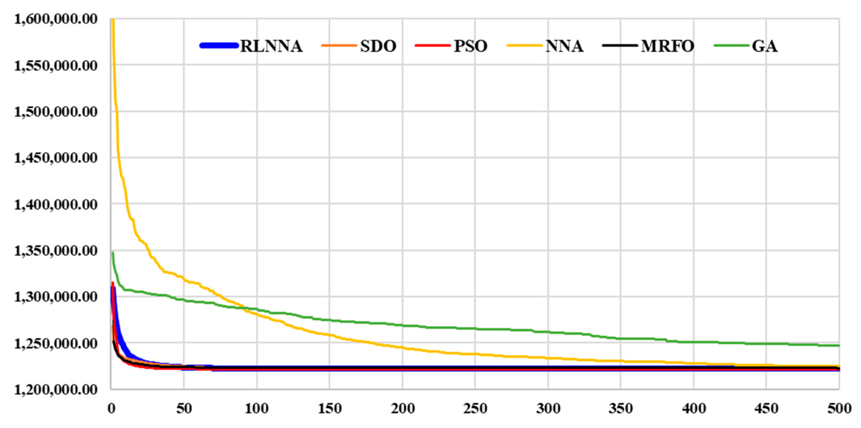
Figure 9 illustrates the convergence rates of the six AI-based techniques—GA, PSO, SDO, NNA, MRFO, and RLNNA. The findings depicted in the figure reveal distinct patterns among the algorithms in terms of their convergence behavior. It is evident from the figure that MRFO, PSO, and SDO exhibit the capability of tracking the optimal global solution. Remarkably, RLNNA demonstrates the fastest convergence among all the algorithms, followed by PSO and SDO. This observation highlights the efficiency of RLNNA in swiftly reaching the optimal solution. On the contrary, GA, and NNA are shown to face challenges in avoiding local solutions and exhibit longer convergence times. The figure indicates that these algorithms may become trapped in local optima, leading to delayed convergence. In conclusion, the analysis of Figure 9 indicates that the RLNNA method performs better than the other five AI techniques for convergence time and global solution capture. The faster convergence of RLNNA, coupled with its capability to follow the optimal global solution, positions it as a promising and effective algorithm for addressing the optimization challenges in the context of the presented computational intelligence-based algorithms.
Table 5 provides a detailed comparison of the optimized parameters generated by different techniques for the microgrid/HES design. The considered AI algorithms include GA, PSO, SDO, RLNNA, NNA, and MRFO. Several key observations highlight the efficacy of RLNNA in comparison to the other AI algorithms:
- ▪
- Superior Economic Optimization:
RLNNA (USD 1,219,744.0) achieves the lowest annualized system cost, showcasing its superior ability to optimize economic parameters.
Versatility: RLNNA demonstrates adaptability in balancing economic feasibility while considering renewable energy integration.
- ▪
- Competitive Renewable Energy Fraction:
RLNNA (86.37%) maintains a competitive REF, emphasizing the algorithm’s ability to balance renewable energy utilization while minimizing costs.
Integrated Approach: RLNNA excels not only in economic optimization but also in considering the ecological impact through effective renewable integration.
- ▪
- Efficient Convergence and Solution Capture:
Convergence Rate: RLNNA exhibits efficient convergence, minimizing the time required to reach optimal solutions.
Global Solution Capture: RLNNA demonstrates effectiveness in capturing global solutions, ensuring well-balanced and reliable hybrid energy system designs.
- ▪
- Algorithmic Robustness:
RLNNA consistently outperforms in achieving the dual objectives of economic optimization and renewable energy integration.
Table 6 presents a comprehensive comparison of optimized parameters derived from the RLNNA algorithm for various hybrid energy system configurations. In the PV/battery/diesel scenario, the power generation is distributed with 5139 kW from PV and 1765 kW from a diesel generator. The system achieves an 83.9% REF with an ASC of USD 1,494,367.8, a surplus energy of 24.9%, and a fuel cost of USD 312,195.5. Conversely, the wind/battery/diesel configuration relies on 4970.5 kW from wind, a battery capacity of 3676.2 kWh, and 2182 kW from a diesel generator. This setup achieves an REF of 65.1%, an ASC of USD 1,593,713.7, a notable surplus energy of 43.0%, and a higher fuel cost of USD 724,655.7. In the PV/wind/diesel scenario, the system incorporates 3100.6 kW from PV, 3863.8 kW from wind, and 1941.8 kW from a diesel generator, resulting in an REF of 78.2%, an ASC of USD 1,454,777.1, a surplus energy of 77.4%, and a fuel cost of USD 547,018.8. Finally, the PV/wind/battery/diesel configuration combines 2990.8 kW from PV, 3025.04 kW from wind, 8290.23 kWh in battery capacity, and 1858.8 kW from a diesel generator, yielding the highest REF at 86.37%, an ASC of USD 1,219,744.0, a surplus energy of 28.1%, and a fuel cost of USD 280,745.5. In comparing these configurations, the PV/wind/battery/diesel system stands out as a well-balanced option, offering high renewable energy utilization, reasonable surplus energy, and competitive costs. These results offer insights into the trade-offs between renewable energy integration, system costs, and surplus energy for each configuration, aiding decision making based on specific objectives and constraints.
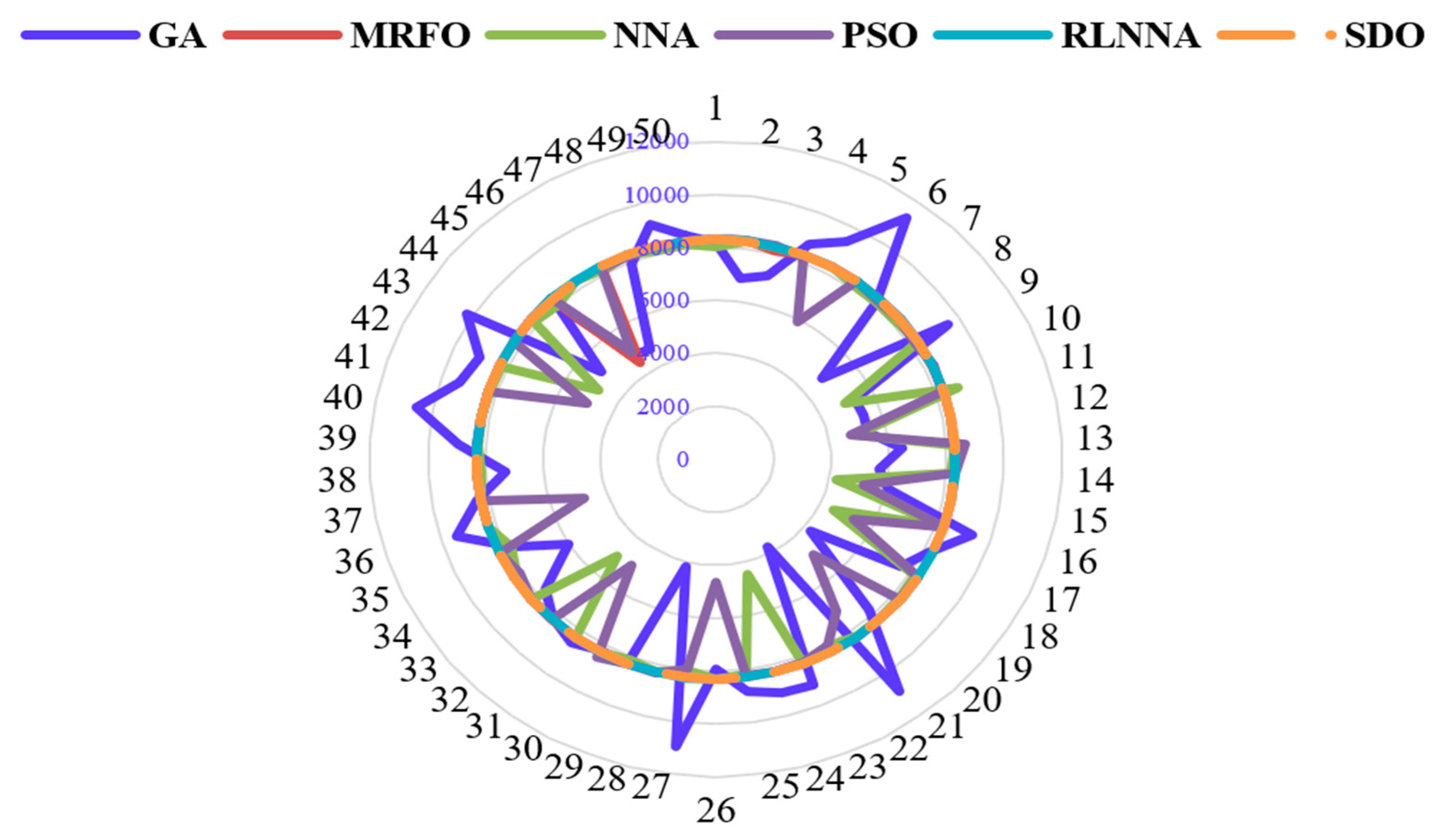
Figure 10 offers crucial insights into the behavior and effectiveness of RLNNA when compared to GA, MRFO, NNA, PSO, and SDO in optimizing battery bank capacities within the examined hybrid energy system (HES).
- ▪
- Competitive Performance: RLNNA, NNA, and PSO exhibit comparable and competitive performance, providing viable alternatives for optimization.
- ▪
- Consistency: SDO, along with MRFO, emerges as a consistently robust performer, showcasing reliable convergence and optimal solutions across multiple runs.
- ▪
- Efficiency: GA displays higher variability and may require further tuning for improved convergence and consistency.
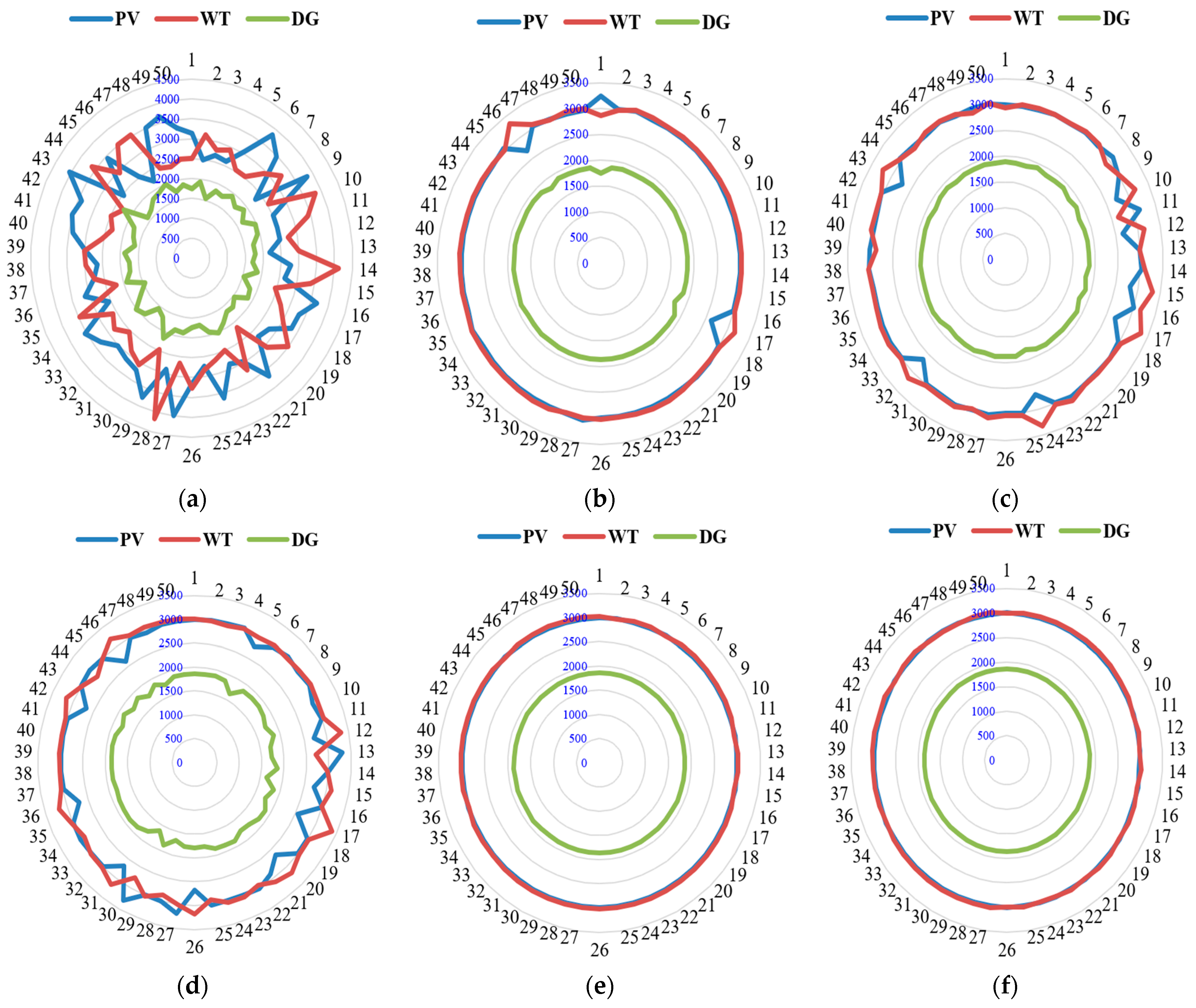
Figure 11 shows the optimal capacities of photovoltaic, wind turbine generators, and diesel in RLNNA when compared to GA, MRFO, NNA, PSO, and SDO over 50 simulation runs. Across these runs, the PV and WT capacities exhibit slight variations, indicating the RLNNA’s ability to consistently suggest optimal solutions. The battery capacity remains relatively stable at approximately 8298.34 kWh, demonstrating the algorithm’s consistent sizing recommendation for the battery bank. Similarly, the diesel generator capacity shows minor fluctuations, ranging between 1857.36 kWh and 1869.03 kWh. These findings collectively highlight the stability and reliability of the RLNNA algorithm in determining optimal component capacities for a hybrid energy system across diverse scenarios.
5. Conclusions
This paper delves into the optimization of microgrid/HESs with a particular focus on sizing configurations that incorporate photovoltaic, wind turbine generators, battery banks, and diesel generators. This study employs a novel soft-computing/metaheuristic algorithm, the reinforcement learning neural network algorithm (RLNNA), to minimize the ASC and enhance system reliability, catering to the energy needs of off-grid areas in Saudi Arabia. The RLNNA algorithm, benchmarked against several other soft-computing algorithms, has demonstrated superior performance regarding faster convergence, capturing optimal global solutions, and minimizing ASC. The results, derived from 50 runs of RLNNA optimization, provide valuable insights into the optimal capacities of key components within HESs. Over the course of the experimentation, RLNNA consistently demonstrated its superior performance, achieving optimal capacities for photovoltaic, wind turbine generators, battery banks, and diesel generators. The comprehensive comparison of algorithms reveals that RLNNA outperforms others regarding both convergence time and global solution capture. Specifically, RLNNA achieves the lowest ASC at USD 1,219,744, showcasing its effectiveness in addressing economic considerations and optimizing system performance. As civilization transitions towards a future dependent on renewable energy, the optimization of HES configurations assumes a more critical role. The RLNNA algorithm, as evidenced by this study, stands as a promising tool for researchers and practitioners alike, offering enhanced efficiency and reliability in the pursuit of sustainable and economically viable off-grid energy solutions. The findings presented herein contribute to the growing body of knowledge in the field, providing a foundation for further exploration and advancement in the optimization of renewable energy conversion systems. For further endeavors, the potential benefits of hybridizing RLNNA with other optimization algorithms should be investigated. Combining the strengths of RLNNA with complementary techniques may yield improved results, especially in addressing multi-objective optimization. This approach could enhance the algorithm’s versatility and robustness across different HES configurations and operational scenarios. The exploration of hybridization strategies presents an exciting avenue for advancing the state of the art in renewable energy system optimization.
Funding
This work was supported and funded by the Deanship of Scientific Research at Imam Mohammad Ibn Saud Islamic University (IMSIU) (grant number IMSIU-RG23030).
Data Availability Statement
The data presented in this study are available on request from the corresponding author.
Conflicts of Interest
The authors declare no conflict of interest.
Nomenclature
| HESs | Hybrid energy systems |
| PV | Photovoltaic |
| WTs | Wind turbines |
| ASC | Annualized system cost |
| LOLE | Loss of load expected |
| LPSP | Loss of power supply probability |
| LOEE | Loss of energy expected |
| LOLH | Loss of load hours |
| DPSP | Deficiency of power supply probability |
| ELF | Equivalent loss factor |
| UL | Unmet load |
| REF | Renewable energy fraction |
| LCC | Life cycle cost |
| COE | Cost of energy |
| NPC | Net present cost |
| RLNNA | Reinforcement learning neural network algorithm |
| PSO | Particle swarm optimization |
| GA | Genetic Algorithm |
| SDO | Supply Demand Optimization |
| MRFO | Manta Ray Foraging Optimization |
| FA | Firefly Algorithm |
| ABS | Artificial Bee Swarm Optimization |
| GAs | Genetic Algorithms |
| CS | Cuckoo search |
| MBA | Mine Blast Algorithm |
| FPA | Flower Pollination Algorithm |
| GOA | Grasshopper Optimization Algorithm |
| ACO | Ant Colony Optimization |
| HHO | Harris Hawk optimization |
References
- Surendra, K.C.; Takara, D.; Hashimoto, A.G.; Khanal, S.K. Biogas as a sustainable energy source for developing countries: Opportunities and challenges. Renew. Sustain. Energy Rev. 2014, 31, 846–859. [Google Scholar] [CrossRef]
- Kamal, M.M.; Mohammad, A.; Ashraf, I.; Fernandez, E. Rural electrification using renewable energy resources and its environmental impact assessment. Environ. Sci. Pollut. Res. 2022, 29, 86562–86579. [Google Scholar] [CrossRef]
- Rathod, A.A.; Subramanian, B. Scrutiny of hybrid renewable energy systems for control, power management, optimization and sizing: Challenges and future possibilities. Sustainability 2022, 14, 16814. [Google Scholar] [CrossRef]
- Alanazi, M.; Alanazi, A.; Almadhor, A.; Rauf, H.T. An Improved Fick’s Law Algorithm Based on Dynamic Lens-Imaging Learning Strategy for Planning a Hybrid Wind/Battery Energy System in Distribution Network. Mathematics 2023, 11, 1270. [Google Scholar] [CrossRef]
- Farh, H.M.; Al-Shamma’a, A.A.; Al-Shaalan, A.M.; Alkuhayli, A.; Noman, A.M.; Kandil, T. Technical and economic evaluation for off-grid hybrid renewable energy system using novel bonobo optimizer. Sustainability 2022, 14, 1533. [Google Scholar] [CrossRef]
- Feron, S. Sustainability of off-grid photovoltaic systems for rural electrification in developing countries: A review. Sustainability 2016, 8, 1326. [Google Scholar] [CrossRef]
- Al-Shamma’a, A.A.; Addoweesh, K.E. Techno-economic optimization of hybrid power system using genetic algorithm. Int. J. Energy Res. 2014, 38, 1608–1623. [Google Scholar] [CrossRef]
- Kvasov, D.E.; Mukhametzhanov, M.S. Metaheuristic vs. deterministic global optimization algorithms: The univariate case. Appl. Math. Comput. 2018, 318, 245–259. [Google Scholar] [CrossRef]
- Dawoud, S.M.; Lin, X.; Okba, M.I. Hybrid renewable microgrid optimization techniques: A review. Renew. Sustain. Energy Rev. 2018, 82, 2039–2052. [Google Scholar] [CrossRef]
- Marini, F.; Walczak, B. Particle swarm optimization (PSO): A tutorial. Chemom. Intell. Lab. Syst. 2015, 149, 153–165. [Google Scholar] [CrossRef]
- Shehab, M.; Khader, A.T.; Al-Betar, M.A. A survey on applications and variants of the cuckoo search algorithm. Appl. Soft Comput. 2017, 61, 1041–1059. [Google Scholar] [CrossRef]
- Khan, B.; Singh, P. Selecting a meta-heuristic technique for smart micro-grid optimization problem: A comprehensive analysis. IEEE Access 2017, 5, 13951–13977. [Google Scholar] [CrossRef]
- Aziz, A.S.; Tajuddin, M.F.N.; Zidane, T.E.K.; Su, C.L.; Mas’ud, A.A.; Alwazzan, M.J.; Alrubaie, A.J.K. Design and optimization of a grid-connected solar energy system: Study in Iraq. Sustainability 2022, 14, 8121. [Google Scholar] [CrossRef]
- Askarzadeh, A. Distribution generation by photovoltaic and diesel generator systems: Energy management and size optimization by a new approach for a stand-alone application. Energy 2017, 122, 542–551. [Google Scholar] [CrossRef]
- Hadidian-Moghaddam, M.J.; Arabi-Nowdeh, S.; Bigdeli, M. Optimal sizing of a stand-alone hybrid photovoltaic/wind system using new grey wolf optimizer considering reliability. J. Renew. Sustain. Energy 2016, 8, 035903. [Google Scholar] [CrossRef]
- Kaabeche, A.; Diaf, S.; Ibtiouen, R. Firefly-inspired algorithm for optimal sizing of renewable hybrid system considering reliability criteria. Sol. Energy 2017, 155, 727–738. [Google Scholar] [CrossRef]
- Maleki, A.; Askarzadeh, A. Artificial bee swarm optimization for optimum sizing of a stand-alone PV/WT/FC hybrid system considering LPSP concept. Sol. Energy 2014, 107, 227–235. [Google Scholar] [CrossRef]
- Ferrari, L.; Bianchini, A.; Galli, G.; Ferrara, G.; Carnevale, E.A. Influence of actual component characteristics on the optimal energy mix of a photovoltaic-wind-diesel hybrid system for a remote off-grid application. J. Clean. Prod. 2018, 178, 206–219. [Google Scholar] [CrossRef]
- Bilal, B.O.; Nourou, D.; Kébé, C.M.F.; Sambou, V.; Ndiaye, P.A.; Ndongo, M. Multi-objective optimization of hybrid PV/wind/diesel/battery systems for decentralized application by minimizing the levelized cost of energy and the CO2 emissions. Int. J. Phys. Sci. 2015, 10, 192–203. [Google Scholar]
- Kaviani, A.K.; Baghaee, H.R.; Riahy, G.H. Optimal sizing of a stand-alone wind/photovoltaic generation unit using particle swarm optimization. Simulation 2009, 85, 89–99. [Google Scholar] [CrossRef]
- Sanchez, V.M.; Chavez-Ramirez, A.U.; Duron-Torres, S.M.; Hernandez, J.; Arriaga, L.G.; Ramirez, J.M. Techno-economical optimization based on swarm intelligence algorithm for a stand-alone wind-photovoltaic-hydrogen power system at south-east region of Mexico. Int. J. Hydrog. Energy 2014, 39, 16646–16655. [Google Scholar] [CrossRef]
- Sharafi, M.; ElMekkawy, T.Y. A dynamic MOPSO algorithm for multiobjective optimal design of hybrid renewable energy systems. Int. J. Energy Res. 2014, 38, 1949–1963. [Google Scholar] [CrossRef]
- Maleki, A.; Askarzadeh, A. Comparative study of artificial intelligence techniques for sizing of a hydrogen-based stand-alone photovoltaic/wind hybrid system. Int. J. Hydrog. Energy 2014, 39, 9973–9984. [Google Scholar] [CrossRef]
- Ghorbani, N.; Kasaeian, A.; Toopshekan, A.; Bahrami, L.; Maghami, A. Optimizing a hybrid wind-PV-battery system using GA-PSO and MOPSO for reducing cost and increasing reliability. Energy 2018, 154, 581–591. [Google Scholar] [CrossRef]
- Fathy, A. A reliable methodology based on mine blast optimization algorithm for optimal sizing of hybrid PV-wind-FC system for remote area in Egypt. Renew. Energy 2016, 95, 367–380. [Google Scholar] [CrossRef]
- Askarzadeh, A. Electrical power generation by an optimised autonomous PV/wind/tidal/battery system. IET Renew. Power Gener. 2017, 11, 152–164. [Google Scholar] [CrossRef]
- Gharibi, M.; Askarzadeh, A. Size and power exchange optimization of a grid-connected diesel generator-photovoltaic-fuel cell hybrid energy system considering reliability, cost and renewability. Int. J. Hydrog. Energy 2019, 44, 25428–25441. [Google Scholar] [CrossRef]
- Zhao, J.; Yuan, X. Multi-objective optimization of stand-alone hybrid PV-wind-diesel-battery system using improved fruit fly optimization algorithm. Soft Comput. 2016, 20, 2841–2853. [Google Scholar] [CrossRef]
- Moghaddam, M.J.H.; Kalam, A.; Nowdeh, S.A.; Ahmadi, A.; Babanezhad, M.; Saha, S. Optimal sizing and energy management of stand-alone hybrid photovoltaic/wind system based on hydrogen storage considering LOEE and LOLE reliability indices using flower pollination algorithm. Renew. Energy 2019, 135, 1412–1434. [Google Scholar] [CrossRef]
- Bukar, A.L.; Tan, C.W.; Lau, K.Y. Optimal sizing of an autonomous photovoltaic/wind/battery/diesel generator microgrid using grasshopper optimization algorithm. Sol. Energy 2019, 188, 685–696. [Google Scholar] [CrossRef]
- Sanajaoba, S.; Fernandez, E. Maiden application of Cuckoo Search algorithm for optimal sizing of a remote hybrid renewable energy system. Renew. Energy 2016, 96, 1–10. [Google Scholar] [CrossRef]
- Shezan, S.A.; Julai, S.; Kibria, M.A.; Ullah, K.R.; Saidur, R.; Chong, W.T.; Akikur, R.K. Performance analysis of an off-grid wind-PV (photovoltaic)-diesel-battery hybrid energy system feasible for remote areas. J. Clean. Prod. 2016, 125, 121–132. [Google Scholar] [CrossRef]
- Baghaee, H.R.; Mirsalim, M.; Gharehpetian, G.B.; Talebi, H.A. Reliability/cost-based multi-objective Pareto optimal design of stand-alone wind/PV/FC generation microgrid system. Energy 2016, 115, 1022–1041. [Google Scholar] [CrossRef]
- Koutroulis, E.; Kolokotsa, D.; Potirakis, A.; Kalaitzakis, K. Methodology for optimal sizing of stand-alone photovoltaic/wind-generator systems using genetic algorithms. Sol. Energy 2006, 80, 1072–1088. [Google Scholar] [CrossRef]
- Eteiba, M.B.; Barakat, S.; Samy, M.M.; Wahba, W.I. Optimization of an off-grid PV/Biomass hybrid system with different battery technologies. Sustain. Cities Soc. 2018, 40, 713–727. [Google Scholar] [CrossRef]
- Sedighizadeh, M.; Esmaili, M.; Esmaeili, M. Application of the hybrid Big Bang-Big Crunch algorithm to optimal reconfiguration and distributed generation power allocation in distribution systems. Energy 2014, 76, 920–930. [Google Scholar] [CrossRef]
- Erdinc, O.; Uzunoglu, M. Optimum design of hybrid renewable energy systems: Overview of different approaches. Renew. Sustain. Energy Rev. 2012, 16, 1412–1425. [Google Scholar] [CrossRef]
- Shi, B.; Wu, W.; Yan, L. Size optimization of stand-alone PV/wind/diesel hybrid power generation systems. J. Taiwan Inst. Chem. Eng. 2017, 73, 93–101. [Google Scholar] [CrossRef]
- Suhane, P.; Rangnekar, S.; Mittal, A.; Khare, A. Sizing and performance analysis of standalone wind-photovoltaic based hybrid energy system using ant colony optimisation. IET Renew. Power Gener. 2016, 10, 964–972. [Google Scholar] [CrossRef]
- Benlahbib, B.; Bouarroudj, N.; Mekhilef, S.; Abdeldjalil, D.; Abdelkrim, T.; Bouchafaa, F. Experimental investigation of power management and control of a PV/wind/fuel cell/battery hybrid energy system microgrid. Int. J. Hydrog. Energy 2020, 45, 29110–29122. [Google Scholar] [CrossRef]
- Shi, Z.; Wang, R.; Zhang, T. Multi-objective optimal design of hybrid renewable energy systems using preference-inspired coevolutionary approach. Sol. Energy 2015, 118, 96–106. [Google Scholar] [CrossRef]
- Jasim, A.M.; Jasim, B.H.; Baiceanu, F.C.; Neagu, B.C. Optimized sizing of energy management system for off-grid hybrid solar/wind/battery/biogasifier/diesel microgrid system. Mathematics 2023, 11, 1248. [Google Scholar] [CrossRef]
- Hadi Abdulwahid, A.; Al-Razgan, M.; Fakhruldeen, H.F.; Churampi Arellano, M.T.; Mrzljak, V.; Arabi Nowdeh, S.; Moghaddam, M.J.H. Stochastic multi-objective scheduling of a hybrid system in a distribution network using a mathematical optimization algorithm considering generation and demand uncertainties. Mathematics 2023, 11, 3962. [Google Scholar] [CrossRef]
- Al-Shamma’a, A.A.; Hussein Farh, H.M.; Noman, A.M.; Al-Shaalan, A.M.; Alkuhayli, A. Optimal Sizing of a Hybrid Renewable Photovoltaic-Wind System-Based Microgrid Using Harris Hawk Optimizer. Int. J. Photoenergy 2022, 2022, 4825411. [Google Scholar] [CrossRef]
- Askarzadeh, A. A discrete chaotic harmony search-based simulated annealing algorithm for optimum design of PV/wind hybrid system. Sol. Energy 2013, 97, 93–101. [Google Scholar] [CrossRef]
- Padrón, I.; Avila, D.; Marichal, G.N.; Rodríguez, J.A. Assessment of Hybrid Renewable Energy Systems to supplied energy to Autonomous Desalination Systems in two islands of the Canary Archipelago. Renew. Sustain. Energy Rev. 2019, 101, 221–230. [Google Scholar] [CrossRef]
- Sadollah, A.; Sayyaadi, H.; Yadav, A. A dynamic metaheuristic optimization model inspired by biological nervous systems: Neural network algorithm. Appl. Soft Comput. 2018, 71, 747–782. [Google Scholar] [CrossRef]
- Zhang, Y. Neural network algorithm with reinforcement learning for parameters extraction of photovoltaic models. IEEE Trans. Neural Netw. Learn. Syst. 2021, 34, 2806–2816. [Google Scholar] [CrossRef]
- Al-Shamma’a, A.A.; Alturki, F.A.; Farh, H.M. Techno-economic assessment for energy transition from diesel-based to hybrid energy system-based off-grids in Saudi Arabia. Energy Transit. 2020, 4, 31–43. [Google Scholar] [CrossRef]
- Givler, T.; Lilienthal, P. Using HOMER Software, NREL’s Micropower Optimization Model, to Explore the Role of Gen-Sets in Small Solar Power Systems Case Study; Technical Report NREL/TP-710-36774, Sri Lanka; National Renewable Energy Lab (NREL): Golden, CO, USA, 2005. [Google Scholar]
- Dehkordi, M.H.R.; Isfahani, A.H.M.; Rasti, E.; Nosouhi, R.; Akbari, M.; Jahangiri, M. Energy-Economic-Environmental assessment of solar-wind-biomass systems for finding the best areas in Iran: A case study using GIS maps. Sustain. Energy Technol. Assess. 2022, 53, 102652. [Google Scholar] [CrossRef]
Figure 1.
The average representation of: (a) The monthly radiation, (b) monthly clearance index, and (c) monthly temperature.
Figure 1.
The average representation of: (a) The monthly radiation, (b) monthly clearance index, and (c) monthly temperature.

Figure 2.
The monthly wind speed (m/s).

Figure 3.
The average monthly load demand in kW.

Figure 4.
Load profile for the city.

Figure 5.
The schematic diagram of the proposed microgrid/HES.

Figure 6.
Framework of the proposed RLNNA.

Figure 7.
Schematic diagram of the RL in RLNNA.

Figure 8.
Pseudo-code of the RLNNA algorithm.

Figure 9.
The RLNNA’s average convergence rate in relation to the other five AI techniques.

Figure 10.
Optimal battery bank capacity vs. runs using GA, MRFO, NNA, PSO, RLNNA, and SDO algorithms.
Figure 10.
Optimal battery bank capacity vs. runs using GA, MRFO, NNA, PSO, RLNNA, and SDO algorithms.

Figure 11.
Optimal capacity of PV, WT, and diesel vs. runs using (a) GA, (b) MRFO, (c) NNA, (d) PSO, (e) RLNNA, and (f) SDO algorithms, respectively.
Figure 11.
Optimal capacity of PV, WT, and diesel vs. runs using (a) GA, (b) MRFO, (c) NNA, (d) PSO, (e) RLNNA, and (f) SDO algorithms, respectively.


Table 1.
Microgrid techno-economic optimization in the literature considering several design factors.
Table 1.
Microgrid techno-economic optimization in the literature considering several design factors.
| Ref. | Microgrid/HES Configurations | Optimization Technique | Technical Objectives and Constraints |
|---|---|---|---|
| [31] | PV/WTs/battery | CS, GA, PSO | ASC, seasonal load variation |
| [14] | PV/diesel | HS | ASC and CO2 |
| [15] | PV/WTs/battery | GWO | ASC, power balance constraints |
| [16] | PV/WTs/battery | FA | COE, load dissatisfaction rate |
| [17] | PV/WTs/FC | ABS | ASC, LPSP |
| [32] | PV/WTs/diesel/battery | HOMER | NPC and CO2 emission |
| [18] | PV/WTs/diesel | GA | ASC, LPSP |
| [20] | PV/WTs/battery | PSO | ASC, full-load demand supply |
| [33] | WTs/PV/FC | PSO | ASC, LOLE, LOEE, ELF |
| [34] | PV/wind/battery | GA | ASC, LOLH |
| [19] | PV/WTs/battery/diesel | GA | COE and CO2 emission |
| [7] | PV/WTs/battery/diesel | GA | COE, REF with zero LPSP |
| [21] | PV/WTs/FC | PSO | NPC and LPSP |
| [22] | PV/wind/diesel/FC/battery | PSO | Multi-objective: UL, NPC, CO2 |
| [23] | PV/WTs/FC | SA, TS, PSO, HS | ASC |
| [24] | PV/battery, WTs/battery, PV/WTs/battery | GA-PSO | NPC and LPSP |
| [25] | PV/WTs/FC | MBA | ASC |
| [26] | PV/WTs/tidal/battery | CSA | NPC, ELF |
| [27] | PV/FC/diesel | CSA | COE and LPSP |
| [28] | PV/WTs/diesel/battery | IFA | ASC and CO2 |
| [35] | PV/Biomass/battery | FPA, ABC, HS, FA | NPC, LPSP, excess energy |
| [36] | PV/wind/battery | BBBC | NPC and UL |
| [37] | PV/diesel | HS | ASC and CO2 |
| [29] | PV/WTs/FC | FPA | NPC, LOLE, LOEE |
| [30] | PV/WTs/battery/diesel | GOA | COE, DPSP |
| [38] | PV/WT/diesel/battery | MLUCA | TAC and GHG emissions minimization |
| [39] | PV/WT/diesel/battery | ACO | Minimize total annual cost (TAC) |
| [40] | PV/WT/diesel/FC/hydrogen tank | MBA | TAC |
| [41] | PV/WT/diesel/battery | PICEA | Minimize ACS, LPSP |
| [42] | PV/WT/bio gasifiers/diesel/battery | GWCSO | Minimize the total cost |
| [43] | PV/WT/battery | IEBSA | Minimizing losses and cost, optimizing the voltage profile, and enhancing ENS |
| [44] | PV/WT/diesel/battery | HHO | ASC minimization |
| [45] | PV/WT/hydrogen/battery | HSSA | Life cycle cost minimization |
| [46] | PV/WT/battery/grid | NN | PLPSP |
Table 2.
Capital, O&M, replacement costs, and lifetime of the microgrid components [49].
Table 2.
Capital, O&M, replacement costs, and lifetime of the microgrid components [49].
| Component | Capital Cost | O&M Cost | Replacement Cost | Lifetime (Years) |
|---|---|---|---|---|
| Photovoltaic | 1000 (USD/kW) | 15 (USD/kW) | - | 20 |
| Wind turbine | 1300 (USD/kW) | 30.33 USD/kW) | - | 20 |
| Battery bank | 200 (USD/kWh) | 5 (USD/kWh) | 200 (USD/kWh) | 5 |
| Diesel generator | 300 (USD/kW) | 0.012 (USD/kWh) | 300 (USD/kW) | 10 |
| Converters | 133 (USD/kW) | 10 (USD/kW) | 100 (USD/kW) | 10 |
Table 3.
The primary characteristics/parameters of the six AI-based algorithms.
| Technique | Characteristic | Value |
|---|---|---|
| Genetic Algorithm (GA) | Population | 100 |
| Selection | Roulette wheel | |
| Rate of mutation | 0.2 | |
| Rate of crossover | 0.8 | |
| Particle Swarm Optimizer (PSO) | Swarm No. | 100 |
| Inertia weight | 1 | |
| Cognitive constant | 0.25 | |
| SDO | Supply weight | 2 |
| Demand weight | 2 | |
| RLNNA | Beta | 1 |
| Bias reduction | 0.99 | |
| NNA | Beta | 1 |
| Bias reduction | 0.99 | |
| MRFO | Constant parameter | α = 1 |
| Somersault factor | 2 | |
| Random numbers r1, r2, r3 | [1 0] |
Table 4.
Performance indicators.
| Algorithm | Performance Indicators (USD/Year) |
Elapsed Time (s) | |||
|---|---|---|---|---|---|
| Optimal | Worst | Mean | STD. | ||
| GA | 1,232,654.5 | 1,280,428.9 | 1,247,373.6 | 10,504.0 | 27.9 |
| PSO | 1,222,098.2 | 1,227,140.5 | 1,222,181.4 | 2081.2 | 41.9 |
| SDO | 1,222,098.2 | 1,222,457.7 | 1,222,166.2 | 68.20 | 47.6 |
| RLNNA | 1,219,744.0 | 1,222,465.4 | 1,221,659.2 | 112.8 | 62.9 |
| NNA | 1,222,319.5 | 1,230,897.2 | 1,224,626.9 | 2388.4 | 27.4 |
| MRFO | 1,222,098.4 | 1,229,389.3 | 1,222,770.8 | 1485.6 | 44.8 |
Table 5.
Optimized parameters generated by the six intelligence-based algorithms.
| Algorithm |
PSolarPV (kW) |
PWind (kW) |
PBattery (kW) |
PDG (kW) |
REF (%) |
ASC (USD/Year) |
Surplus (%) |
Fuel Cost (USD/Year) |
|---|---|---|---|---|---|---|---|---|
| GA | 3217.1 | 3051.47 | 8257.17 | 1697.9 | 87.11 | 1,232,654.5 | 32.2 | 257,866.9 |
| PSO | 2990.8 | 3025.03 | 8290.23 | 1858.9 | 86.37 | 1,222,098.2 | 28.0 | 280,896.4 |
| SDO | 2990.8 | 3025.03 | 8290.23 | 1858.8 | 86.33 | 1,222,098.2 | 28.0 | 280,745.4 |
| RLNNA | 2990.8 | 3025.04 | 8290.23 | 1858.8 | 86.37 | 1,219,744.0 | 28.1 | 280,745.5 |
| NNA | 2989.3 | 3023.27 | 8296.33 | 1858.1 | 86.36 | 1,222,319.5 | 28.0 | 281,080.6 |
| MRFO | 2990.8 | 3025.02 | 8290.26 | 1858.9 | 86.41 | 1,222,098.4 | 28.1 | 281,015.5 |
Table 6.
Optimized parameters of four HESs generated by the RLNNA algorithm.
| Configuration |
PPV (kW) |
PWT (kW) |
PBatt (kWh) |
PDG (kW) |
REF (%) |
ASC (USD/Year) |
Surplus (%) |
Fuel Cost (USD/Year) |
|---|---|---|---|---|---|---|---|---|
| PV/Battery/Diesel | 5139 | 0 | 18661.7 | 1765 | 83.9 | 1,494,367.8 | 24.9 | 312,195.5 |
| Wind/Battery/Diesel | 0 | 4970.5 | 3676.2 | 2182 | 65.1 | 1,593,713.7 | 43.0 | 724,655.7 |
| PV/Wind/Diesel | 3100.6 | 3863.8 | 0 | 1941.8 | 78.2 | 1,454,777.1 | 77.4 | 547,018.8 |
| PV/Wind/Battery/Diesel | 2990.8 | 3025.04 | 8290.23 | 1858.8 | 86.37 | 1,219,744.0 | 28.1 | 280,745.5 |
Disclaimer/Publisher’s Note: The statements, opinions and data contained in all publications are solely those of the individual author(s) and contributor(s) and not of MDPI and/or the editor(s). MDPI and/or the editor(s) disclaim responsibility for any injury to people or property resulting from any ideas, methods, instructions or products referred to in the content. |
© 2024 by the author. Licensee MDPI, Basel, Switzerland. This article is an open access article distributed under the terms and conditions of the Creative Commons Attribution (CC BY) license (https://creativecommons.org/licenses/by/4.0/).
Share and Cite
MDPI and ACS Style
Hussein Farh, H.M. Neural Network Algorithm with Reinforcement Learning for Microgrid Techno-Economic Optimization. Mathematics 2024, 12, 280. https://doi.org/10.3390/math12020280
AMA Style
Hussein Farh HM. Neural Network Algorithm with Reinforcement Learning for Microgrid Techno-Economic Optimization. Mathematics. 2024; 12(2):280. https://doi.org/10.3390/math12020280
Chicago/Turabian StyleHussein Farh, Hassan M. 2024. "Neural Network Algorithm with Reinforcement Learning for Microgrid Techno-Economic Optimization" Mathematics 12, no. 2: 280. https://doi.org/10.3390/math12020280
Note that from the first issue of 2016, this journal uses article numbers instead of page numbers. See further details here.